Creates an elegant alluvial/Sankey diagram showing how items flow from one set of categories to another. Useful for visualizing cluster transitions, state changes, or any categorical mapping.
Usage
plot_transitions(
  x,
  from_title = "From",
  to_title = "To",
  title = NULL,
  from_colors = NULL,
  to_colors = NULL,
  flow_fill = "#888888",
  flow_alpha = 0.4,
  flow_color_by = NULL,
  flow_border = NA,
  flow_border_width = 0.5,
  node_width = 0.08,
  node_border = NA,
  node_spacing = 0.02,
  label_size = 3.5,
  label_position = c("beside", "inside", "above", "below", "outside"),
  mid_label_position = NULL,
  label_halo = TRUE,
  label_color = "black",
  label_fontface = "plain",
  label_nudge = 0.02,
  title_size = 5,
  title_color = "black",
  title_fontface = "bold",
  curve_strength = 0.6,
  show_values = FALSE,
  value_position = c("center", "origin", "destination", "outside_origin",
    "outside_destination"),
  value_size = 3,
  value_color = "black",
  value_halo = NULL,
  value_fontface = "bold",
  value_nudge = 0.03,
  value_min = 0,
  show_totals = FALSE,
  total_size = 4,
  total_color = "white",
  total_fontface = "bold",
  conserve_flow = TRUE,
  min_flow = 0,
  threshold = 0,
  value_digits = 2,
  column_gap = 1,
  track_individuals = FALSE,
  line_alpha = 0.3,
  line_width = 0.5,
  jitter_amount = 0.8,
  proportional_nodes = TRUE,
  node_label_format = NULL,
  bundle_size = NULL,
  bundle_legend = TRUE,
  bundle_legend_size = 3,
  bundle_legend_color = "grey50",
  bundle_legend_fontface = "italic",
  bundle_legend_position = c("bottom", "top")
)
Arguments
- x
Input data in one of several formats:
A transition matrix (rows = from, cols = to, values = counts)
Two vectors: pass
beforeas x andafteras second argument (contingency table computed automatically, like chi-square)A 2-column data frame (raw observations; table computed automatically)
A data frame with columns: from, to, count
A list of matrices for multi-step transitions
- from_title
Title for the left column. Default "From". For multi-step, use a vector of titles (e.g., c("T1", "T2", "T3", "T4")).
- to_title
Title for the right column. Default "To". Ignored for multi-step.
- title
Optional plot title. Applied via ggplot2::labs(title = title).
- from_colors
Colors for left-side nodes. Default uses palette.
- to_colors
Colors for right-side nodes. Default uses palette.
- flow_fill
Fill color for flows. Default "#888888" (grey). In multi-step and individual-tracking plots, ignored when
flow_color_byis set; simple two-column aggregate plots useflow_fill.- flow_alpha
Alpha transparency for flows. Default 0.4.
- flow_color_by
Color flows by state. For multi-step aggregate flows, use
"source"or"destination"; for individual trajectories,"first"and"last"are also supported. Default NULL usesflow_fill; simple two-column aggregate plots ignore this argument.- flow_border
Border color for flows. Default NA (no border).
- flow_border_width
Line width for flow borders. Default 0.5.
- node_width
Width of node rectangles (0-1 scale). Default 0.08.
- node_border
Border color for nodes. Default NA (no border).
- node_spacing
Vertical spacing between nodes (0-1 scale). Default 0.02.
- label_size
Size of node labels. Default 3.5.
- label_position
Position of node labels: "beside" (default), "inside", "above", "below", "outside". Applied to first and last columns. See
mid_label_positionfor middle columns.- mid_label_position
Position of labels for intermediate (middle) columns in individual-tracking plots. Same options as
label_position. Default NULL useslabel_positionvalue.- label_halo
Logical: add white halo around labels for readability? Default TRUE.
- label_color
Color of state name labels. Default "black". Applied to multi-step and individual-tracking plots; simple two-column aggregate plots use black external labels and white inside labels.
- label_fontface
Font face of state name labels ("plain", "bold", "italic", "bold.italic"). Default "plain". Applied to multi-step and individual-tracking plots; simple two-column aggregate plots use fixed label font faces.
- label_nudge
Distance between node edge and label (in plot units). Default 0.02. Used by multi-step and individual-tracking plots.
- title_size
Size of column titles. Default 5.
- title_color
Color of column title text. Default "black". Applied to multi-step and individual-tracking plots; simple two-column aggregate plots use black titles.
- title_fontface
Font face of column titles. Default "bold". Applied to multi-step and individual-tracking plots.
- curve_strength
Controls bezier curve shape (0-1). Default 0.6.
- show_values
Logical: show transition counts on flows? Default FALSE.
- value_position
Position of flow values: "center", "origin", "destination", "outside_origin", "outside_destination". Default "center".
- value_size
Size of value labels on flows. Default 3.
- value_color
Color of value labels. Default "black".
- value_halo
Logical: add halo around flow value labels? Default NULL (inherits from
label_halo). Applied to multi-step and individual-tracking plots.- value_fontface
Font face of flow value labels. Default "bold". Applied to multi-step and individual-tracking plots.
- value_nudge
Distance of value labels from node edge when using "origin" or "destination" positions. Default 0.03.
- value_min
Minimum count to show a flow value label in multi-step and individual-tracking plots. Default 0 (show all). Simple two-column aggregate plots show all nonzero value labels when
show_values = TRUE.- show_totals
Logical: show total counts on nodes? Default FALSE.
- total_size
Size of total labels. Default 4.
- total_color
Color of total labels. Default "white".
- total_fontface
Font face of total labels. Default "bold".
- conserve_flow
Logical: should left and right totals match? Default TRUE. When FALSE, each side scales independently (allows for "lost" or "gained" items).
- min_flow
Minimum flow value to display. Default 0 (show all).
- threshold
Minimum edge weight to display. Flows below this value are removed. Combined with
min_flow: effective minimum ismax(threshold, min_flow). Default 0.- value_digits
Number of decimal places for flow value labels and node totals. Default 2.
- column_gap
Horizontal spread of columns (0-1) for multi-step and individual-tracking plots. Default 1 uses full width. Use smaller values (e.g., 0.6) to bring columns closer together.
- track_individuals
Logical: draw individual lines instead of aggregated flows? Default FALSE. When TRUE, each row in the data frame becomes a separate line.
- line_alpha
Alpha for individual tracking lines. Default 0.3.
- line_width
Width of individual tracking lines. Default 0.5.
- jitter_amount
Vertical jitter for individual lines (0-1). Default 0.8.
- proportional_nodes
Logical: size nodes proportionally to counts in individual-tracking plots? Default TRUE.
- node_label_format
Format string for node labels with
{state}and{count}placeholders in individual-tracking plots. Default NULL (plain state name). Example:"{state} (n={count})".- bundle_size
Controls line bundling for large datasets. Default NULL (no bundling). Integer >= 2: each drawn line represents that many cases. Numeric in (0,1): reduce to this fraction of original lines (e.g., 0.15 keeps about 15 percent of lines).
- bundle_legend
Logical or character: show annotation when bundling is active? Default TRUE shows "Each line ~ N cases" below the plot. Pass a string to use custom text (with
{n}placeholder for count).- bundle_legend_size
Size of the bundle legend text. Default 3.
- bundle_legend_color
Color of the bundle legend text. Default "grey50".
- bundle_legend_fontface
Font face of the bundle legend text. Default "italic".
- bundle_legend_position
Position of the bundle legend: "bottom" (default) or "top".
Details
The function creates smooth bezier curves connecting nodes from the left column to the right column. Flow width is proportional to the transition count. Nodes are sized proportionally to their total flow.
Examples
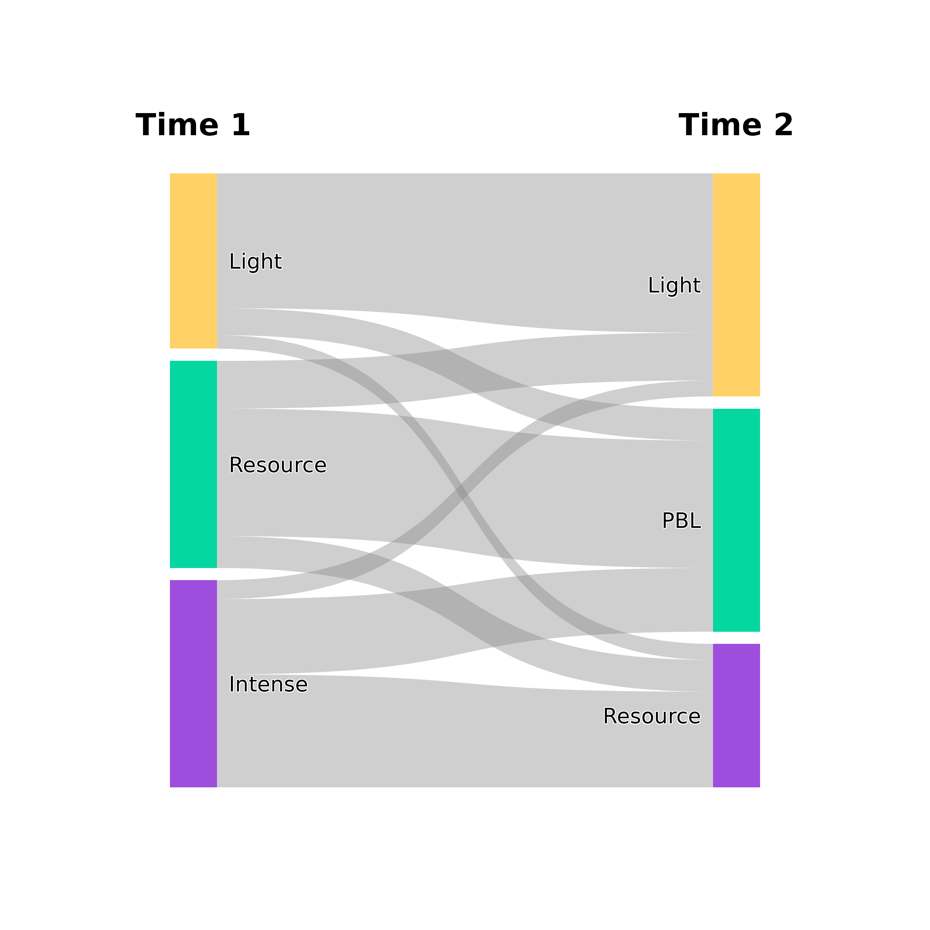
# From a transition matrix
mat <- matrix(c(50, 10, 5, 15, 40, 10, 5, 20, 30), 3, 3, byrow = TRUE,
dimnames = list(c("Light","Resource","Intense"),
c("Light","PBL","Resource")))
plot_transitions(mat, from_title = "Time 1", to_title = "Time 2")
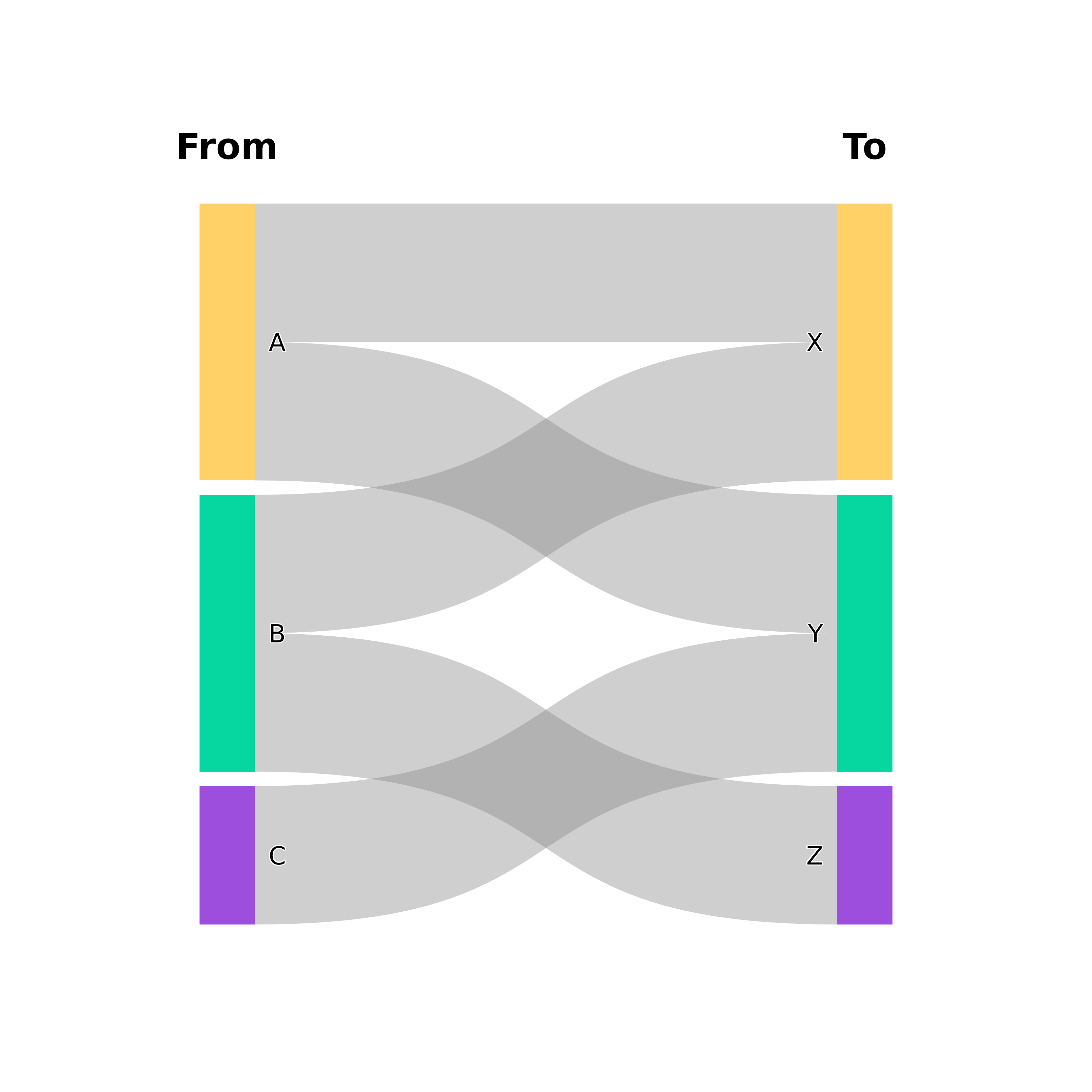
 # From a 2-column data frame (auto-contingency)
df <- data.frame(time1 = c("A","A","B","B","C"),
time2 = c("X","Y","X","Z","Y"))
plot_transitions(df)
# From a 2-column data frame (auto-contingency)
df <- data.frame(time1 = c("A","A","B","B","C"),
time2 = c("X","Y","X","Z","Y"))
plot_transitions(df)