Why cograph?
Mohammed Saqr and Sonsoles López-Pernas
Source:vignettes/articles/why-cograph.Rmd
why-cograph.RmdDo we need another network package?
R already has igraph for computation and qgraph for psychometric networks. tidygraph tries to unify things with a dplyr grammar. So why write another one?
The short answer: none of these packages let you go from a raw matrix to a filtered, annotated, publication-ready figure without switching between ecosystems, reformatting objects, or writing boilerplate. cograph tries to close that gap.
This document walks through the specific things cograph does differently, with working examples.
Filtering and selecting — like data frames
In igraph, subsetting a network means calling
induced_subgraph(), delete_edges(), or
indexing into V(g) and E(g). In tidygraph, you
need activate(nodes) |> filter(...). Both approaches
require you to think about the object structure.
cograph lets you filter nodes and edges with expressions that look
like subset():
mat <- matrix(c(
  0.0, 0.5, 0.8, 0.1, 0.0,
  0.3, 0.0, 0.2, 0.6, 0.4,
  0.7, 0.1, 0.0, 0.3, 0.5,
  0.0, 0.4, 0.2, 0.0, 0.9,
  0.1, 0.3, 0.6, 0.8, 0.0
), 5, 5, byrow = TRUE)
rownames(mat) <- colnames(mat) <- c("Read", "Write", "Plan", "Code", "Test")
net <- as_cograph(mat)
Keep only edges above a threshold:
strong <- filter_edges(net, weight > 0.5)
get_edges(strong)
#>   from to weight
#> 1    3  1    0.7
#> 2    1  3    0.8
#> 3    5  3    0.6
#> 4    2  4    0.6
#> 5    5  4    0.8
#> 6    4  5    0.9
Keep nodes that have high degree and high PageRank — the centrality measures are computed on the fly:
hubs <- filter_nodes(net, degree >= 3 & pagerank > 0.15)
get_nodes(hubs)
#>   id label  name  x  y
#> 1  1  Read  Read NA NA
#> 2  2 Write Write NA NA
#> 3  3  Plan  Plan NA NA
#> 4  4  Code  Code NA NA
#> 5  5  Test  Test NA NA
Structural selections
select_nodes() goes further. It knows about components,
neighborhoods, articulation points, and k-cores — and it computes them
lazily (only what your expression actually references):
# Top 3 nodes by betweenness
top3 <- select_top(net, n = 3, by = "betweenness")
get_nodes(top3)
#>   id label  name  x  y
#> 1  1 Write Write NA NA
#> 2  2  Plan  Plan NA NA
#> 3  3  Code  Code NA NA
# Ego network: everything within 1 hop of "Code"
ego <- select_neighbors(net, of = "Code", order = 1)
get_nodes(ego)
#>   id label  name  x  y
#> 1  1  Read  Read NA NA
#> 2  2 Write Write NA NA
#> 3  3  Plan  Plan NA NA
#> 4  4  Code  Code NA NA
#> 5  5  Test  Test NA NA
For edges, you can select by structure too:
# Edges involving "Code"
code_edges <- select_edges_involving(net, nodes = "Code")
get_edges(code_edges)
#>   from to weight
#> 1    4  2    0.4
#> 2    4  3    0.2
#> 3    1  4    0.1
#> 4    2  4    0.6
#> 5    3  4    0.3
#> 6    5  4    0.8
#> 7    4  5    0.9
# Top 5 edges by weight
top5 <- select_top_edges(net, n = 5)
get_edges(top5)
#>   from to weight
#> 1    3  1    0.7
#> 2    1  3    0.8
#> 3    5  3    0.6
#> 4    5  4    0.8
#> 5    4  5    0.9
# Edges between two node sets
between <- select_edges_between(net,
  set1 = c("Read", "Write"),
  set2 = c("Code", "Test")
)
get_edges(between)
#>   from to weight
#> 1    5  1    0.1
#> 2    4  2    0.4
#> 3    5  2    0.3
#> 4    1  4    0.1
#> 5    2  4    0.6
#> 6    2  5    0.4
Format in, same format out
If you pass a matrix, you can get a matrix back:
filter_edges(mat, weight > 0.5, keep_format = TRUE)
#>       Read Write Plan Code Test
#> Read   0.0     0  0.8  0.0  0.0
#> Write  0.0     0  0.0  0.6  0.0
#> Plan   0.7     0  0.0  0.0  0.0
#> Code   0.0     0  0.0  0.0  0.9
#> Test   0.0     0  0.6  0.8  0.0
Same for igraph objects. No lock-in.
Centrality — one call, tidy table
igraph requires a separate function for each centrality measure, and
each returns a different format. page_rank(g) gives you a
list with $vector. betweenness(g) gives a
named numeric. Building a comparison table takes 10+ lines.
In cograph, one call with the built-in edge-list data returns a tidy centrality table:
data(student_interactions)
centrality(student_interactions)
#>    node degree_all strength_all closeness_all betweenness  eigenvector
#> 1    Ac         33          129    0.01754386   26.342857 1.000000e+00
#> 2    Ad         20           36    0.01754386   42.541520 1.096110e-01
#> 3    Fi         24           51    0.01666667   35.721634 1.789565e-01
#> 4    Ik         14           24    0.01666667   25.844874 1.551369e-02
#> 5    Vx         26           43    0.01960784   90.717124 7.238902e-02
#> 6    Rt         20           37    0.01785714   63.135739 1.159931e-01
#> 7    Km         11           16    0.01639344   18.175108 2.804725e-02
#> 8    Gj         19           31    0.01818182  114.599049 3.265786e-02
#> 9    Bd         12           18    0.01612903   21.769264 9.607736e-03
#> 10   Ce         10           13    0.01612903   16.648629 4.473504e-03
#> 11   Oq         14           20    0.01754386   34.151726 2.293068e-02
#> 12   Ya         13           19    0.01612903   18.216122 1.758656e-02
#> 13   Mo         12           17    0.01587302   38.264502 1.003629e-01
#> 14   Hj         12           19    0.01754386   85.816522 2.013125e-02
#> 15   Tv         10           13    0.01666667   25.916306 1.320877e-02
#> 16   Eg         10           12    0.01639344   22.335171 5.783916e-03
#> 17   Pr         11           18    0.01666667   23.974060 7.602231e-02
#> 18   Qs         15           19    0.01785714   76.910851 1.511764e-02
#> 19   Xz         14           18    0.01639344   22.280159 8.533484e-03
#> 20   Np          8            8    0.01666667   12.044048 1.549052e-02
#> 21   Dg         13           13    0.01886792   29.240901 6.260099e-03
#> 22   Hk         16           25    0.01818182   72.176441 1.201845e-01
#> 23   Wy         11           16    0.01639344   34.014358 1.054705e-03
#> 24   Jl         15           18    0.01818182   67.359085 5.009801e-02
#> 25   Fh         21           55    0.01818182   78.588877 2.817489e-01
#> 26   Zb          7            8    0.01538462    9.583333 5.429715e-05
#> 27   Eh          7           13    0.01428571   34.325000 1.163185e-03
#> 28   Be         14           16    0.01851852  105.250898 2.203252e-03
#> 29   Df          8           10    0.01562500   11.026190 4.800876e-06
#> 30   Cf         12           15    0.01724138  119.109163 1.243207e-02
#> 31   Su          6            9    0.01369863   33.154401 1.028472e-04
#> 32   Ln          7            8    0.01408451    5.749708 1.376854e-02
#> 33   Gi          3            4    0.01351351    0.000000 0.000000e+00
#> 34   Uw          4            7    0.01250000    0.000000 0.000000e+00
#>       pagerank
#> 1  0.285861728
#> 2  0.052985644
#> 3  0.077591140
#> 4  0.024836857
#> 5  0.057364714
#> 6  0.042552472
#> 7  0.016655998
#> 8  0.025444498
#> 9  0.014321668
#> 10 0.010679742
#> 11 0.016087378
#> 12 0.016588876
#> 13 0.031180263
#> 14 0.019051413
#> 15 0.012644206
#> 16 0.010425091
#> 17 0.022794289
#> 18 0.019784870
#> 19 0.013229134
#> 20 0.008466679
#> 21 0.010345027
#> 22 0.040383192
#> 23 0.009067435
#> 24 0.020529375
#> 25 0.070538086
#> 26 0.005635780
#> 27 0.010080122
#> 28 0.009378924
#> 29 0.004957518
#> 30 0.017877547
#> 31 0.005136500
#> 32 0.007628879
#> 33 0.005483193
#> 34 0.004411765
That includes degree, strength, closeness, betweenness, eigenvector centrality, and PageRank. No igraph conversion, no transition-matrix helper, no wrapper.
Less common measures are available through the same wrapper style:
centrality_harmonic(student_interactions)
#>       Ac       Ad       Fi       Ik       Vx       Rt       Km       Gj
#> 21.33333 21.66667 20.50000 20.16667 24.00000 21.50000 19.66667 22.00000
#>       Bd       Ce       Oq       Ya       Mo       Hj       Tv       Eg
#> 19.50000 19.50000 21.66667 20.16667 19.33333 21.33333 19.83333 20.00000
#>       Pr       Qs       Xz       Np       Dg       Hk       Wy       Jl
#> 19.83333 21.83333 20.33333 20.16667 23.00000 22.00000 20.00000 22.33333
#>       Fh       Zb       Eh       Be       Df       Cf       Su       Ln
#> 22.00000 18.33333 16.83333 22.50000 18.83333 20.83333 16.33333 17.33333
#>       Gi       Uw
#> 15.83333 14.83333
Need just one measure as a named vector? Use the wrapper:
centrality_pagerank(student_interactions)
#>          Ac          Ad          Fi          Ik          Vx          Rt
#> 0.285861728 0.052985644 0.077591140 0.024836857 0.057364714 0.042552472
#>          Km          Gj          Bd          Ce          Oq          Ya
#> 0.016655998 0.025444498 0.014321668 0.010679742 0.016087378 0.016588876
#>          Mo          Hj          Tv          Eg          Pr          Qs
#> 0.031180263 0.019051413 0.012644206 0.010425091 0.022794289 0.019784870
#>          Xz          Np          Dg          Hk          Wy          Jl
#> 0.013229134 0.008466679 0.010345027 0.040383192 0.009067435 0.020529375
#>          Fh          Zb          Eh          Be          Df          Cf
#> 0.070538086 0.005635780 0.010080122 0.009378924 0.004957518 0.017877547
#>          Su          Ln          Gi          Uw
#> 0.005136500 0.007628879 0.005483193 0.004411765
centrality_betweenness(student_interactions)
#>         Ac         Ad         Fi         Ik         Vx         Rt         Km
#>  26.342857  42.541520  35.721634  25.844874  90.717124  63.135739  18.175108
#>         Gj         Bd         Ce         Oq         Ya         Mo         Hj
#> 114.599049  21.769264  16.648629  34.151726  18.216122  38.264502  85.816522
#>         Tv         Eg         Pr         Qs         Xz         Np         Dg
#>  25.916306  22.335171  23.974060  76.910851  22.280159  12.044048  29.240901
#>         Hk         Wy         Jl         Fh         Zb         Eh         Be
#>  72.176441  34.014358  67.359085  78.588877   9.583333  34.325000 105.250898
#>         Df         Cf         Su         Ln         Gi         Uw
#>  11.026190 119.109163  33.154401   5.749708   0.000000   0.000000
You can normalize, sort, and round in the same call:
centrality(student_interactions, normalized = TRUE,
           sort_by = "pagerank", digits = 3)
#>    node degree_all strength_all closeness_all betweenness eigenvector pagerank
#> 1    Ac      1.000        1.000         0.579       0.221       1.000    1.000
#> 2    Fi      0.727        0.395         0.550       0.300       0.179    0.271
#> 3    Fh      0.636        0.426         0.600       0.660       0.282    0.247
#> 4    Vx      0.788        0.333         0.647       0.762       0.072    0.201
#> 5    Ad      0.606        0.279         0.579       0.357       0.110    0.185
#> 6    Rt      0.606        0.287         0.589       0.530       0.116    0.149
#> 7    Hk      0.485        0.194         0.600       0.606       0.120    0.141
#> 8    Mo      0.364        0.132         0.524       0.321       0.100    0.109
#> 9    Gj      0.576        0.240         0.600       0.962       0.033    0.089
#> 10   Ik      0.424        0.186         0.550       0.217       0.016    0.087
#> 11   Pr      0.333        0.140         0.550       0.201       0.076    0.080
#> 12   Jl      0.455        0.140         0.600       0.566       0.050    0.072
#> 13   Qs      0.455        0.147         0.589       0.646       0.015    0.069
#> 14   Hj      0.364        0.147         0.579       0.720       0.020    0.067
#> 15   Cf      0.364        0.116         0.569       1.000       0.012    0.063
#> 16   Km      0.333        0.124         0.541       0.153       0.028    0.058
#> 17   Ya      0.394        0.147         0.532       0.153       0.018    0.058
#> 18   Oq      0.424        0.155         0.579       0.287       0.023    0.056
#> 19   Bd      0.364        0.140         0.532       0.183       0.010    0.050
#> 20   Xz      0.424        0.140         0.541       0.187       0.009    0.046
#> 21   Tv      0.303        0.101         0.550       0.218       0.013    0.044
#> 22   Ce      0.303        0.101         0.532       0.140       0.004    0.037
#> 23   Eg      0.303        0.093         0.541       0.188       0.006    0.036
#> 24   Dg      0.394        0.101         0.623       0.245       0.006    0.036
#> 25   Eh      0.212        0.101         0.471       0.288       0.001    0.035
#> 26   Be      0.424        0.124         0.611       0.884       0.002    0.033
#> 27   Wy      0.333        0.124         0.541       0.286       0.001    0.032
#> 28   Np      0.242        0.062         0.550       0.101       0.015    0.030
#> 29   Ln      0.212        0.062         0.465       0.048       0.014    0.027
#> 30   Zb      0.212        0.062         0.508       0.080       0.000    0.020
#> 31   Gi      0.091        0.031         0.446       0.000       0.000    0.019
#> 32   Su      0.182        0.070         0.452       0.278       0.000    0.018
#> 33   Df      0.242        0.078         0.516       0.093       0.000    0.017
#> 34   Uw      0.121        0.054         0.413       0.000       0.000    0.015
Edge-level centrality
edge_centrality(net, sort_by = "betweenness", digits = 3)
#>     from    to weight betweenness overlap shared_neighbors triangles
#> 1   Code  Plan    0.2         8.0       1                3         3
#> 2   Read  Code    0.1         7.0       1                3         3
#> 3   Plan Write    0.1         6.5       1                3         3
#> 4  Write  Read    0.3         4.0       1                3         3
#> 5   Test  Read    0.1         3.0       1                3         3
#> 6  Write  Test    0.4         2.5       1                3         3
#> 7   Plan  Test    0.5         1.5       1                3         3
#> 8  Write  Plan    0.2         1.0       1                3         3
#> 9   Plan  Code    0.3         1.0       1                3         3
#> 10  Test Write    0.3         1.0       1                3         3
#> 11  Read Write    0.5         0.0       1                3         3
#> 12  Read  Plan    0.8         0.0       1                3         3
#> 13 Write  Code    0.6         0.0       1                3         3
#> 14  Plan  Read    0.7         0.0       1                3         3
#> 15  Code Write    0.4         0.0       1                3         3
#> 16  Code  Test    0.9         0.0       1                3         3
#> 17  Test  Plan    0.6         0.0       1                3         3
#> 18  Test  Code    0.8         0.0       1                3         3
#>    reciprocated reverse_weight weight_ratio
#> 1          TRUE            0.3        1.500
#> 2         FALSE             NA           NA
#> 3          TRUE            0.2        2.000
#> 4          TRUE            0.5        1.667
#> 5         FALSE             NA           NA
#> 6          TRUE            0.3        0.750
#> 7          TRUE            0.6        1.200
#> 8          TRUE            0.1        0.500
#> 9          TRUE            0.2        0.667
#> 10         TRUE            0.4        1.333
#> 11         TRUE            0.3        0.600
#> 12         TRUE            0.7        0.875
#> 13         TRUE            0.4        0.667
#> 14         TRUE            0.8        1.143
#> 15         TRUE            0.6        1.500
#> 16         TRUE            0.8        0.889
#> 17         TRUE            0.5        0.833
#> 18         TRUE            0.9        1.125
Network-level summary
One-row data frame with density, diameter, transitivity, centralization, reciprocity, and more:
network_summary(net, digits = 3)
#>   node_count edge_count density component_count diameter mean_distance min_cut
#> 1          5         18     0.9               1      0.8          0.35       3
#>   centralization_degree centralization_in_degree centralization_out_degree
#> 1                 0.125                      0.1                       0.1
#>   centralization_betweenness centralization_closeness centralization_eigen
#> 1                      0.028                        0                0.097
#>   transitivity reciprocity assortativity_degree
#> 1        1.009         0.8                -0.25
Add detailed = TRUE for mean/sd of node-level measures,
or extended = TRUE for girth, radius, global efficiency,
etc.
Community detection — one call
igraph has cluster_louvain(),
cluster_walktrap(), etc. — different function per
algorithm, inconsistent parameter names. cograph wraps all of them
behind one function with a default:
# Undirected network for community detection
sym <- (mat + t(mat)) / 2
diag(sym) <- 0
cograph::communities(sym)
#> Community structure (louvain)
#>   Nodes: 5  | Communities: 2  | Modularity: 0.0985
#>   Sizes: 2, 3
#>
#>   node community
#>   Read         1
#>  Write         2
#>   Plan         1
#>   Code         2
#>   Test         2
Pick a different algorithm by name, or use two-letter shorthands:
cograph::communities(sym, method = "walktrap")
#> Community structure (walktrap)
#>   Nodes: 5  | Communities: 2  | Modularity: 0.0985
#>   Sizes: 2, 3
#>
#>   node community
#>   Read         1
#>  Write         2
#>   Plan         1
#>   Code         2
#>   Test         2
com_fg(sym)   # fast greedy
#> Community structure (fast_greedy)
#>   Nodes: 5  | Communities: 2  | Modularity: 0.0985
#>   Sizes: 3, 2
#>
#>   node community
#>   Read         2
#>  Write         1
#>   Plan         2
#>   Code         1
#>   Test         1
com_im(mat)   # infomap (works on directed too)
#> Community structure (infomap)
#>   Nodes: 5  | Communities: 1  | Modularity: 0
#>   Sizes: 5
#>
#>   node community
#>   Read         1
#>  Write         1
#>   Plan         1
#>   Code         1
#>   Test         1
If you just want a node-to-community data frame:
detect_communities(sym, method = "walktrap")
#> Community structure (walktrap)
#>   Nodes: 5  | Communities: 2  | Modularity: 0.0985
#>   Sizes: 2, 3
#>
#>   node community
#>   Read         1
#>  Write         2
#>   Plan         1
#>   Code         2
#>   Test         2
Quality and significance
How good is the partition?
comm <- com_wt(mat)
det <- detect_communities(mat, method = "walktrap")
cluster_list <- split(det$node, det$community)
cqual(mat, cluster_list)
#> Cluster Quality Metrics
#> =======================
#>
#> Global metrics:
#>   Modularity: 0
#>   Coverage:   1
#>   Clusters:   1
#>
#> Per-cluster metrics:
#>  cluster cluster_name n_nodes internal_edges cut_edges internal_density
#>        1            1       5            7.8         0             0.39
#>  avg_internal_degree expansion cut_ratio conductance
#>                 3.12         0        NA           0
Is the modularity significantly higher than chance? Permutation test against a null model:
csig(mat, comm, n_random = 200, seed = 1)
#> Cluster Significance Test
#> =========================
#>
#>   Null model:           configuration (n = 200 )
#>   Observed modularity:  0
#>   Null mean:            0.1787
#>   Null SD:              0.0953
#>   Z-score:              -1.88
#>   P-value:              0.96961
#>
#>   Conclusion: No significant community structure (p >= 0.05)
Compare two solutions
comm2 <- com_fg(mat)
compare_communities(comm, comm2, method = "nmi")
#> [1] 0
Consensus clustering
Run a stochastic algorithm many times and threshold the co-occurrence matrix:
com_consensus(mat, method = "infomap", n_runs = 50, seed = 1)
#> Community structure (consensus_infomap)
#>   Nodes: 5  | Communities: 1  | Modularity: 0
#>   Sizes: 5
#>
#>   node community
#>   Read         1
#>  Write         1
#>   Plan         1
#>   Code         1
#>   Test         1
Format interoperability
cograph accepts matrices, edge lists, igraph, statnet, qgraph, and tna objects natively. And it converts back:
net <- as_cograph(mat)

# To igraph
g <- to_igraph(net)
class(g)
#> [1] "igraph"

# To matrix
m <- to_matrix(net)
m[1:3, 1:3]
#>       Read Write Plan
#> Read   0.0   0.5  0.8
#> Write  0.3   0.0  0.2
#> Plan   0.7   0.1  0.0

# To edge list
head(to_df(net))
#>    from    to weight
#> 1 Write  Read    0.3
#> 2  Plan  Read    0.7
#> 3  Test  Read    0.1
#> 4  Read Write    0.5
#> 5  Plan Write    0.1
#> 6  Code Write    0.4
No format lock-in. Use cograph for what it’s good at, convert back when you need something else.
Robustness, motifs, backbone
A few more things that would otherwise require separate packages:
Robustness analysis
How does the network hold up when you remove nodes by betweenness (targeted attack) vs. random failure?
rob <- robustness(mat, measure = "betweenness", strategy = "sequential", seed = 1)
rob_rand <- robustness(mat, measure = "random", n_iter = 50, seed = 1)

# Area under curve — higher means more robust
robustness_auc(rob)
#> [1] 0.5
robustness_auc(rob_rand)
#> [1] 0.5
Disparity filter (backbone extraction)
Keep only edges that carry a disproportionate share of a node’s weight:
backbone <- disparity_filter(mat, level = 0.5)
backbone
#>       Read Write Plan Code Test
#> Read     0     1    1    0    0
#> Write    0     0    0    1    1
#> Plan     1     0    0    0    1
#> Code     0     1    0    0    1
#> Test     0     1    1    1    0
Motif census
Count triad types with significance testing against a configuration model:
motif_census(mat, n_random = 100)
#> Network Motif Analysis
#> Size: 3-node motifs (directed) | Null: configuration (n=100)
#>
#>  motif count null_mean null_sd z_score p_value significant
#>    003     0         0       0       0       1       FALSE
#>    012     0         0       0       0       1       FALSE
#>    102     0         0       0       0       1       FALSE
#>   021D     0         0       0       0       1       FALSE
#>   021U     0         0       0       0       1       FALSE
#>   021C     0         0       0       0       1       FALSE
#>   111D     0         0       0       0       1       FALSE
#>   111U     0         0       0       0       1       FALSE
#>   030T     0         0       0       0       1       FALSE
#>   030C     0         0       0       0       1       FALSE
#>    201     0         0       0       0       1       FALSE
#>   120D     0         0       0       0       1       FALSE
#>   120U     0         0       0       0       1       FALSE
#>   120C     1         1       0       0       1       FALSE
#>    210     4         4       0       0       1       FALSE
#>    300     5         5       0       0       1       FALSE
#>
#> Over-represented: 0 | Under-represented: 0
Working with probabilistic networks
cograph was built with transition networks in mind — matrices where rows sum to 1 and edges are probabilities, not just weights. This matters in a few places.
Smart weight inversion
Path-based centrality measures (betweenness, closeness, harmonic) need distances, not probabilities. For transition networks, a high-probability edge should mean short distance. cograph handles this automatically:
- For tna objects: weights are inverted (distance = 1/probability)
- For other networks: weights are used as-is (standard igraph convention)
No manual toggle needed.
First-class tna support
If you use the tna package for Transition Network Analysis, cograph understands its objects directly:
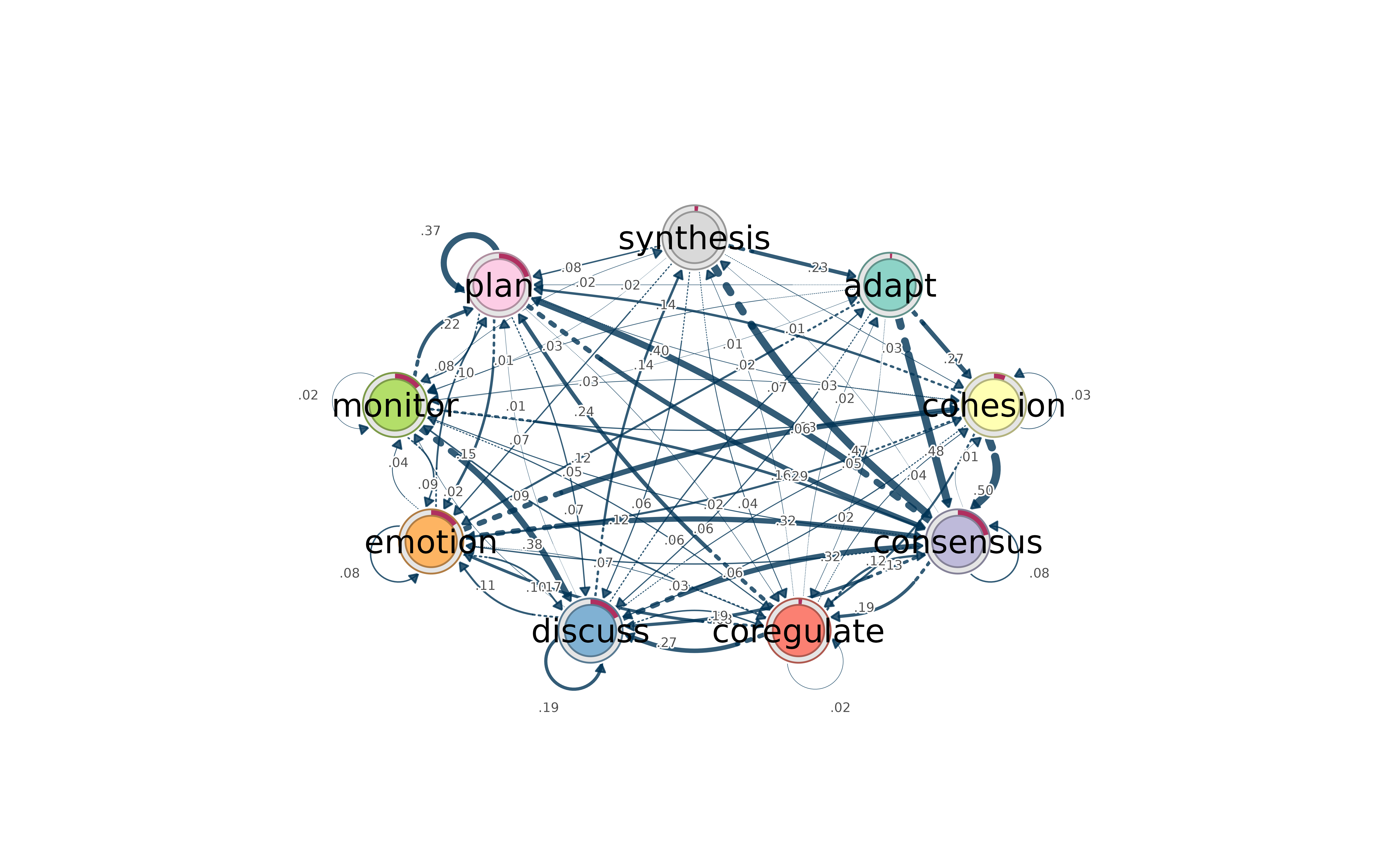
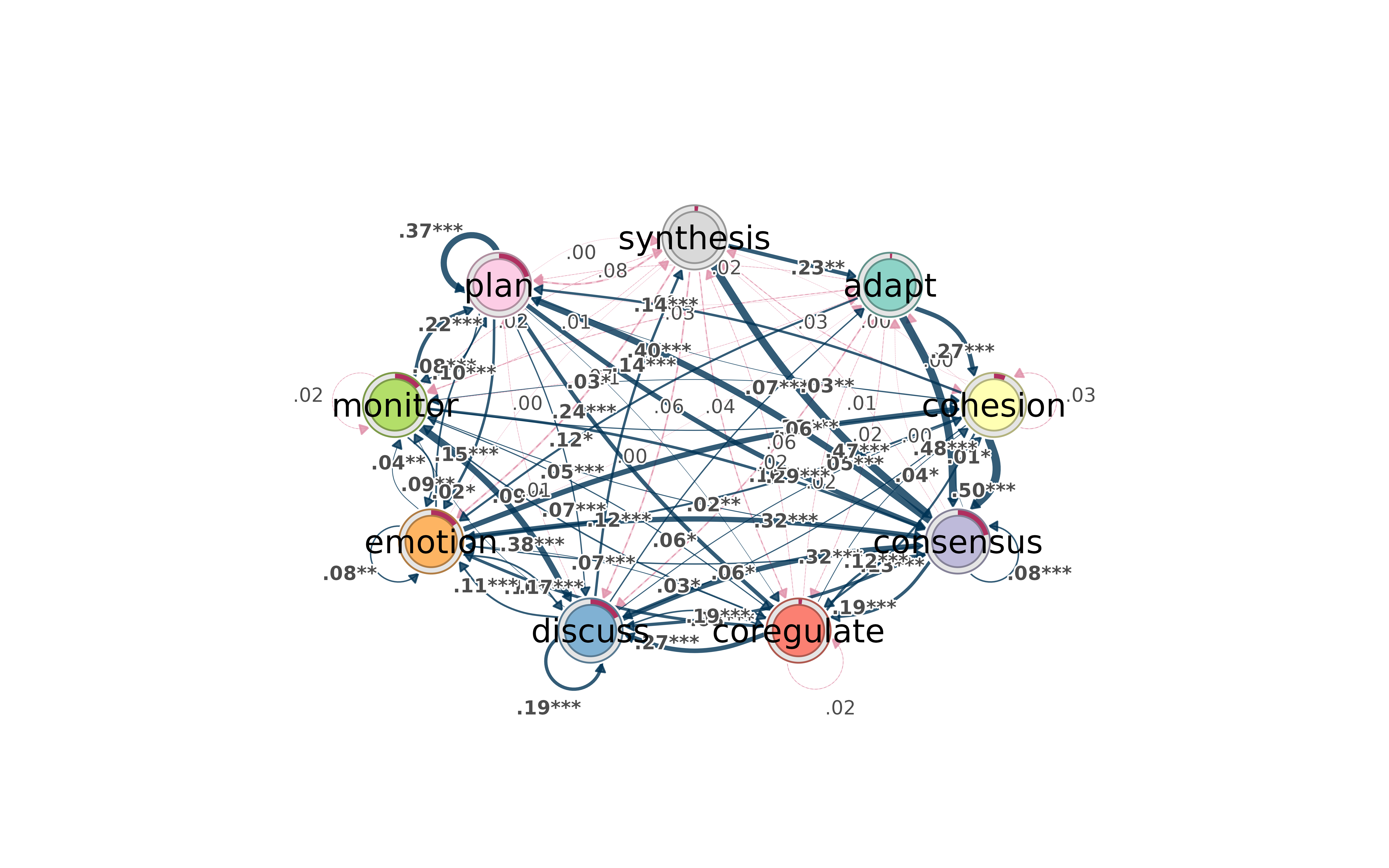
Bootstrap results render automatically — significant transitions as solid edges, non-significant as dashed:
Permutation test results get color-coded by group effect:
model1 <- tna(group_regulation[1:1000,])
model2 <- tna(group_regulation[1001:2000,])

perm <- permutation_test(model1, model2, iter = 1000)
splot(perm)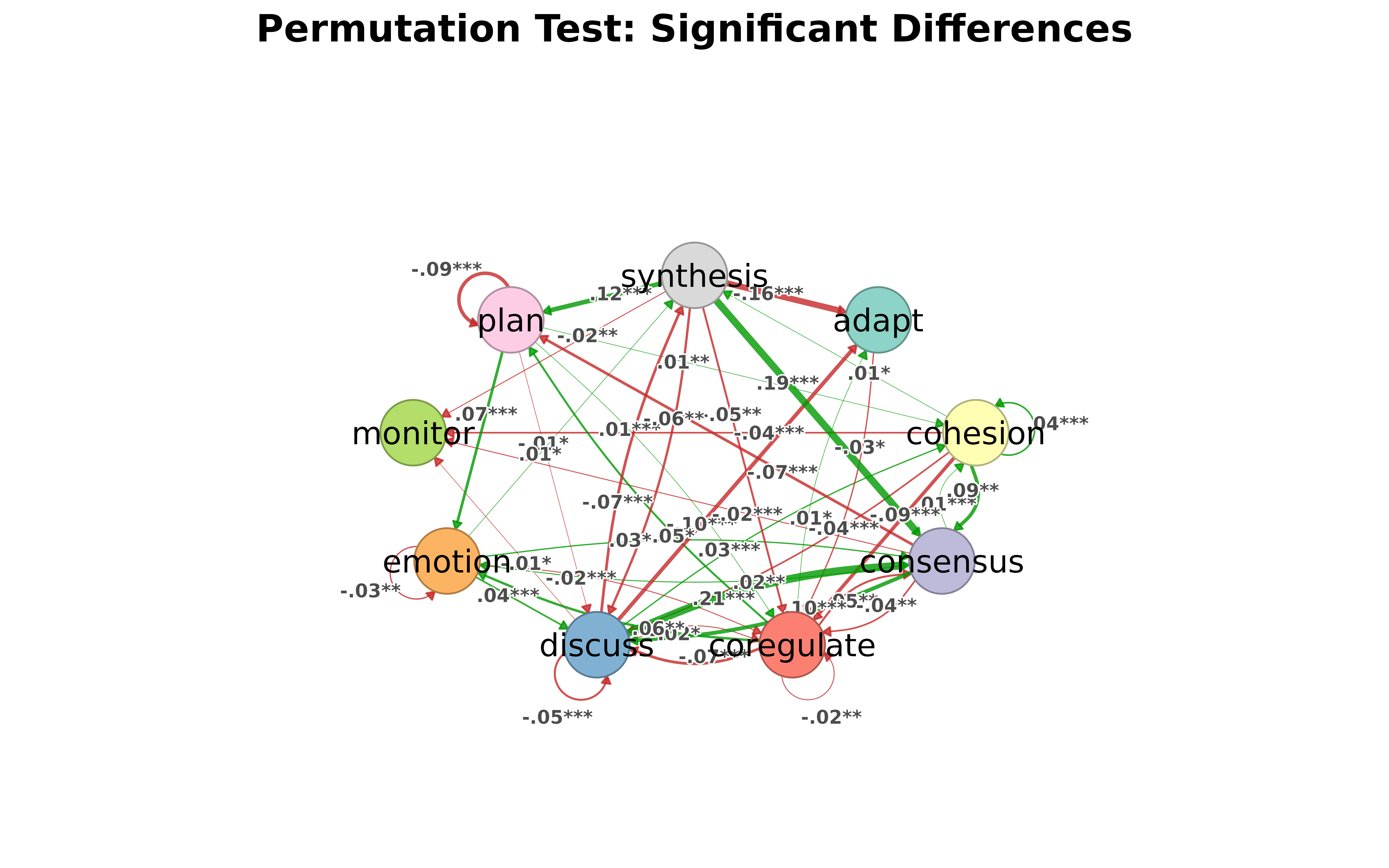
Group comparisons with plot_compare() show element-wise
probability differences, with donuts on nodes for initial state
shifts.
qgraph compatibility
Researchers coming from qgraph can use familiar parameter names —
vsize, asize, edge.color, etc. —
they are translated automatically. When both the cograph name and the
qgraph alias are present, the cograph name wins.
Nestimate integration
cograph also plots Nestimate objects (bootstrap forests, permutation results, glasso networks) without importing the package — dispatch is by class name only.
Summary
cograph is not trying to replace igraph’s graph algorithms or tidygraph’s data manipulation. It fills a different gap: going from data to a filtered, annotated, publication-ready network figure with minimal code, while staying interoperable with everything else in the R network ecosystem.
The main ideas:
- Filter and select with data-frame-like expressions, not object-specific APIs
- Centrality as a tidy data frame, not a list of separate calls
- Community detection behind one function with shorthands, quality metrics, and significance tests
- Statistical annotation (CIs, p-values, stars) directly on the figure
- No format lock-in — matrix/igraph/statnet/tna in and out
- Probabilistic networks handled correctly out of the box