Sequence pattern comparison: early vs late Human-AI interactions • htna

A transition network represents the joint distribution of single-step state transitions, marginalising over higher-order structure. When the analytic question concerns recurring multi-step patterns — fixed-length subsequences (k-grams) such as Command -> Specify -> Execute — single-step summaries are insufficient: they decompose the pattern into independent steps and lose its identity as a unit.

sequence_compare_htna() operates at the k-gram level. For two or more cohorts of sessions, the function enumerates every k-gram of length within a specified range (e.g. Request -> Specify -> Execute), computes the per-cohort frequency, and tests whether the pattern’s rate differs across cohorts under either a chi-square or a permutation null model. Standardised residuals identify which cohort each pattern characterises.

The example below applies the procedure to a between-session split: sessions are ranked chronologically by their first session_date (ties broken on session_id), the first half of sessions are labelled "Early", and the rest "Late". The analytic question is which patterns characterise the early phase of the corpus’s lifetime and which characterise the late phase.

Data preparation

The bundled human_ai corpus already carries an actor_type column distinguishing Human and AI events (see ?human_ai). The session-level phase column marks each session as "Early" or "Late" based on its rank in chronological order.

library(htna)
data(human_ai)

table(human_ai$phase)
#> 
#> Early  Late 
#> 10170  9177

Constructing the grouped htna network

build_htna() accepts both actor_type (the within-session actor partition) and group (the between-session cohort grouping) simultaneously. The result is an object of class htna_group: a named list of htna networks, one per cohort, each carrying the actor partition. Cohort labels are read by sequence_compare_htna() from the list names; no separate group argument is required at the comparison step.

net_g <- build_htna(
  human_ai,
  actor_type = "actor_type",
  group      = "phase"
)
class(net_g)
#> [1] "htna_group"      "netobject_group" "list"
names(net_g)
#> [1] "Late"  "Early"

Pattern comparison

sequence_compare_htna() is invoked on the grouped network. Pattern lengths 3 to 5 are scanned; only patterns occurring at least 25 times across the corpus are retained. The permutation test is used because each session belongs to exactly one cohort, so the exchangeability assumption that underlies the permutation null is satisfied. False-discovery-rate correction (adjust = "fdr") controls for multiple testing across the candidate patterns.

res <- sequence_compare_htna(
  net_g,
  sub      = 3:5,
  min_freq = 25L,
  test     = "permutation",
  adjust   = "fdr"
)
res
#> Sequence Comparison  [106 patterns | 2 groups: Early, Late]
#>   Lengths: 3, 4, 5  |  min_freq: 25  |  permutation: 1000 iter (fdr)
#> 
#>                                      pattern length freq_Early freq_Late
#>                        Request->Specify->Ask      3        147       197
#>  Execute->Request->Execute->Request->Execute      5         35        56
#>                    Specify->Request->Specify      3         82       116
#>                         Ask->Plan->Frustrate      3         74       112
#>       Request->Specify->Frustrate->Ask->Plan      5        105        51
#>                  Request->Specify->Ask->Plan      4         68        91
#>         Request->Request->Specify->Frustrate      4         85        40
#>                Specify->Frustrate->Ask->Plan      4        106        51
#>                  Request->Specify->Frustrate      3        160        88
#>                       Plan->Request->Execute      3        114        61
#>   prop_Early   prop_Late resid_Early resid_Late effect_size    p_value
#>  0.015089304 0.022519433   -3.733134   3.733134    5.422831 0.01512773
#>  0.003756574 0.006729960   -2.751564   2.751564    4.707396 0.01512773
#>  0.008417163 0.013260174   -3.194473   3.194473    4.650011 0.01512773
#>  0.007595976 0.012802926   -3.542427   3.542427    4.499102 0.01512773
#>  0.011269722 0.006129071    3.640078  -3.640078    4.425205 0.01512773
#>  0.007136111 0.010663229   -2.533619   2.533619    4.321670 0.01512773
#>  0.008920139 0.004687134    3.426113  -3.426113    3.832168 0.01512773
#>  0.011123937 0.005976096    3.721097  -3.721097    4.809739 0.01925347
#>  0.016423732 0.010059442    3.756080  -3.756080    4.582489 0.01925347
#>  0.011701909 0.006973022    3.315762  -3.315762    3.801624 0.01925347
#>   ... and 96 more patterns

The discriminative patterns appear at the top of the patterns table, ranked by test statistic.

head(res$patterns, 10)
#>                                        pattern length freq_Early freq_Late
#> 1                        Request->Specify->Ask      3        147       197
#> 2  Execute->Request->Execute->Request->Execute      5         35        56
#> 3                    Specify->Request->Specify      3         82       116
#> 4                         Ask->Plan->Frustrate      3         74       112
#> 5       Request->Specify->Frustrate->Ask->Plan      5        105        51
#> 6                  Request->Specify->Ask->Plan      4         68        91
#> 7         Request->Request->Specify->Frustrate      4         85        40
#> 8                Specify->Frustrate->Ask->Plan      4        106        51
#> 9                  Request->Specify->Frustrate      3        160        88
#> 10                      Plan->Request->Execute      3        114        61
#>     prop_Early   prop_Late resid_Early resid_Late effect_size    p_value
#> 1  0.015089304 0.022519433   -3.733134   3.733134    5.422831 0.01512773
#> 2  0.003756574 0.006729960   -2.751564   2.751564    4.707396 0.01512773
#> 3  0.008417163 0.013260174   -3.194473   3.194473    4.650011 0.01512773
#> 4  0.007595976 0.012802926   -3.542427   3.542427    4.499102 0.01512773
#> 5  0.011269722 0.006129071    3.640078  -3.640078    4.425205 0.01512773
#> 6  0.007136111 0.010663229   -2.533619   2.533619    4.321670 0.01512773
#> 7  0.008920139 0.004687134    3.426113  -3.426113    3.832168 0.01512773
#> 8  0.011123937 0.005976096    3.721097  -3.721097    4.809739 0.01925347
#> 9  0.016423732 0.010059442    3.756080  -3.756080    4.582489 0.01925347
#> 10 0.011701909 0.006973022    3.315762  -3.315762    3.801624 0.01925347

Interpreting the standardised residuals

For each pattern, the standardised residual is computed from a 2×2 contingency table of (this pattern present vs. all other patterns) crossed with cohort:

$\text{stdres}_{ij} = \frac{O_{ij} - E_{ij}}{\sqrt{E_{ij} \cdot (1 - r_i / N) \cdot (1 - c_j / N)}}$

A positive residual on the Early cohort indicates that the pattern is over-represented in sessions from the first half of the corpus’s lifetime; a positive residual on the Late cohort indicates over-representation in sessions from the second half. By the standardised-residual interpretation, $|z| > 1.96$ corresponds to $p < 0.05$ at the cell level, and $|z| > 3$ provides strong evidence of over- or under-representation.

Pyramid display

The pyramid display arranges the top patterns as back-to-back horizontal bars, with each cohort on one side. Bar length encodes the per-cohort frequency; the in-bar label gives the standardised residual. The colour scale is shared across both sides so that residuals are directly comparable.

plot(res, style = "pyramid", show_residuals = TRUE)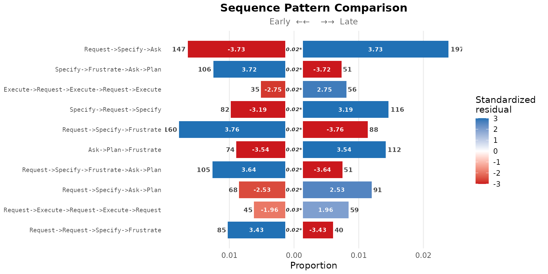

The pyramid display requires exactly two cohorts and is the most direct visual comparison when this condition is met.

Heatmap display

The heatmap display generalises to any number of cohorts. Each column is a cohort; each row is a pattern; cell colour encodes the standardised residual under the same scale as the pyramid display.

plot(res, style = "heatmap")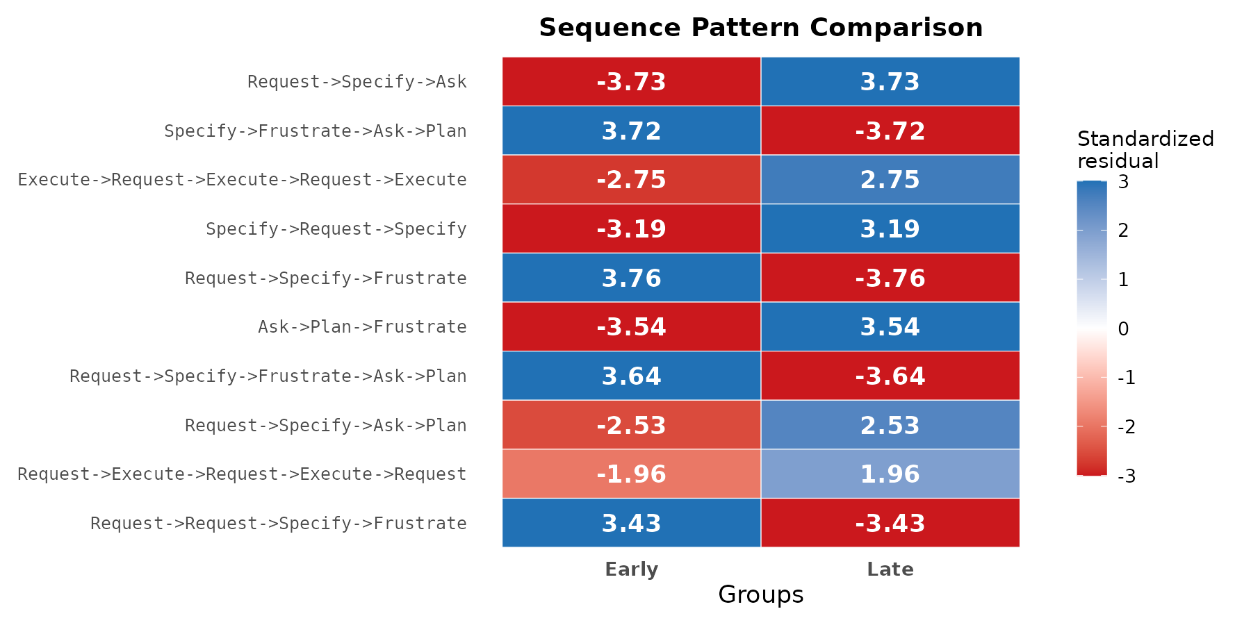

Sorting by frequency

By default, patterns are ranked by the test statistic — the most discriminative patterns appear first. Ranking by total occurrence count is alternative when the analytic interest is on the most common patterns regardless of their cohort difference.

plot(res, style = "pyramid", sort = "frequency", show_residuals = TRUE)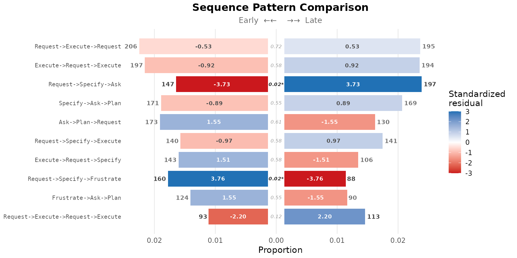

Meta-path comparison (actor-type level)

By default, sequence_compare_htna() enumerates k-grams over the concrete state codes. Setting level = "type" first folds each state into its actor type before pattern enumeration, so the comparison runs on meta-paths such as Human -> AI -> Human rather than concrete state sequences. This collapses the alphabet to the actor partition and surfaces which cohort is characterised by particular handover structures between actor types, independent of the specific codes involved.

level = "type" requires x to be an htna network carrying an actor partition ($node_groups) — net_g above qualifies because build_htna() was given actor_type = "actor_type".

res_type <- sequence_compare_htna(
  net_g,
  level    = "type",
  sub      = 3:5,
  min_freq = 25L,
  test     = "permutation",
  adjust   = "fdr"
)
res_type
#> Sequence Comparison  [52 patterns | 2 groups: Early, Late]
#>   Lengths: 3, 4, 5  |  min_freq: 25  |  permutation: 1000 iter (fdr)
#> 
#>                         pattern length freq_Early freq_Late  prop_Early
#>  Human->Human->Human->AI->Human      5        112       196 0.012021037
#>  AI->Human->Human->Human->Human      5         41        71 0.004400558
#>            Human->Human->AI->AI      4        846       646 0.088781614
#>                   Human->AI->AI      3       1203       986 0.123485937
#>     Human->Human->Human->AI->AI      5        315       228 0.033809166
#>     Human->Human->AI->AI->Human      5        676       525 0.072555544
#>     Human->Human->AI->Human->AI      5        323       345 0.034667812
#>            Human->AI->AI->Human      4        976       796 0.102424179
#>        AI->AI->Human->AI->Human      5        363       279 0.038961039
#>                Human->AI->Human      3       1813      1780 0.186101417
#>    prop_Late resid_Early resid_Late effect_size    p_value
#>  0.023554861   -5.837799   5.837799    7.371409 0.05194805
#>  0.008532628   -3.448798   3.448798    4.064398 0.05194805
#>  0.075697211    3.189261  -3.189261    3.651386 0.05194805
#>  0.112711477    2.264188  -2.264188    2.684103 0.12750885
#>  0.027400553    2.459688  -2.459688    2.602828 0.12750885
#>  0.063093378    2.490338  -2.490338    2.579126 0.12750885
#>  0.041461363   -2.359490   2.359490    2.466456 0.12750885
#>  0.093273963    2.064052  -2.064052    2.356914 0.12750885
#>  0.033529624    1.922749  -1.922749    2.342807 0.12750885
#>  0.203475080   -2.980988   2.980988    2.279054 0.12750885
#>   ... and 42 more patterns

plot(res_type, style = "pyramid", show_residuals = TRUE)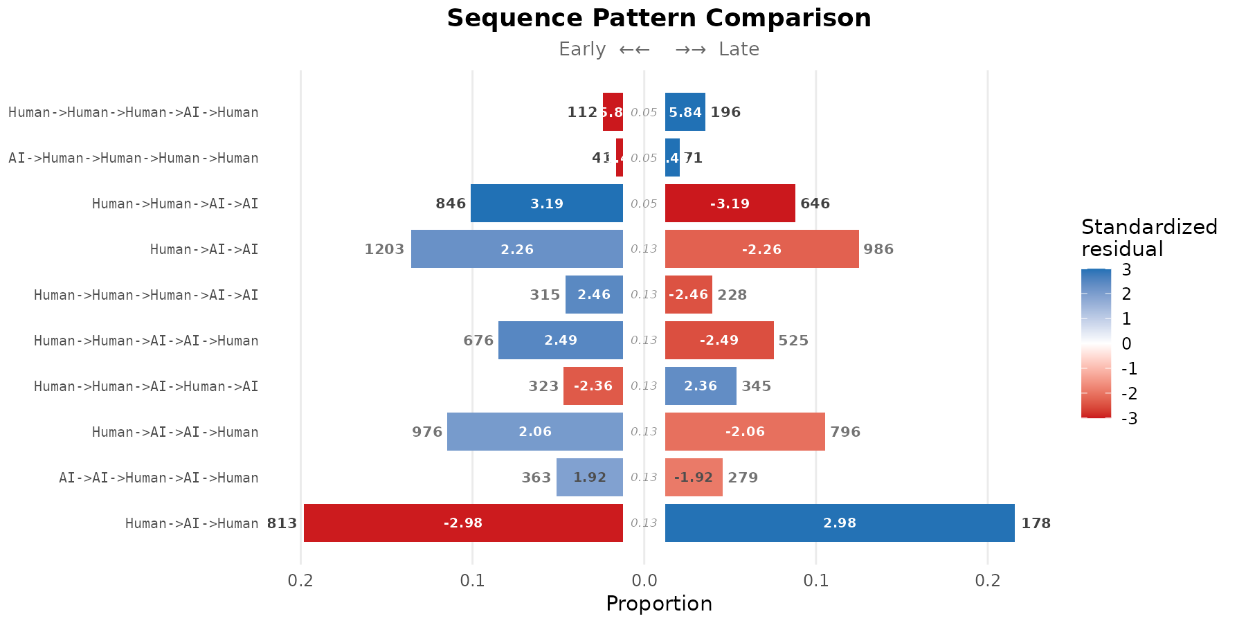

Choice of test statistic

The two test choices supported by sequence_compare_htna() correspond to different assumptions about the source of the sessions in each cohort.

Permutation (test = "permutation") shuffles cohort labels at the session level and assumes exchangeability across sessions. It is appropriate when the cohorts comprise independent groups of sessions — for example, sessions from different time periods, projects, or experimental conditions — as in the chronological split used here.
Chi-square (test = "chisq") tests independence between pattern and cohort in the pooled contingency table. It assumes the underlying counts come from independent observations and is fast — useful as a default when cohorts comprise independent sessions and per-cell pattern counts are large enough for the asymptotic χ² approximation to hold. It is not appropriate when the same units contribute to multiple cohorts.

Selection of the test should follow from the design that produced the cohort labels.