Getting Started with htna • htna

Heterogeneous Transition Network Analysis (HTNA) studies sequences in which two or more actors interleave – a learner and a tutor, a human and an AI, a clinician and a patient – and treats each actor’s codes as a distinct node group. The htna package builds the network, computes the usual analytical quantities, and renders the result with the actor partition baked into colour, layout, and the legend.

1. Building a heterogeneous network

Start from one long-format data frame with an actor-type column tagging each row ("Human" or "AI") and pass its name as actor_type to build_htna(). The result is a network whose nodes carry the actor label they came from. The bundled human_ai corpus (see ?human_ai) is used throughout this vignette.

library(htna)
data(human_ai)

net <- build_htna(human_ai, actor_type = "actor_type", actor = "session_id")

2. Plotting the network

plot_htna() lays out actor groups around the circle, colours each node by its actor type, and draws the actor legend below the plot:

plot_htna(net)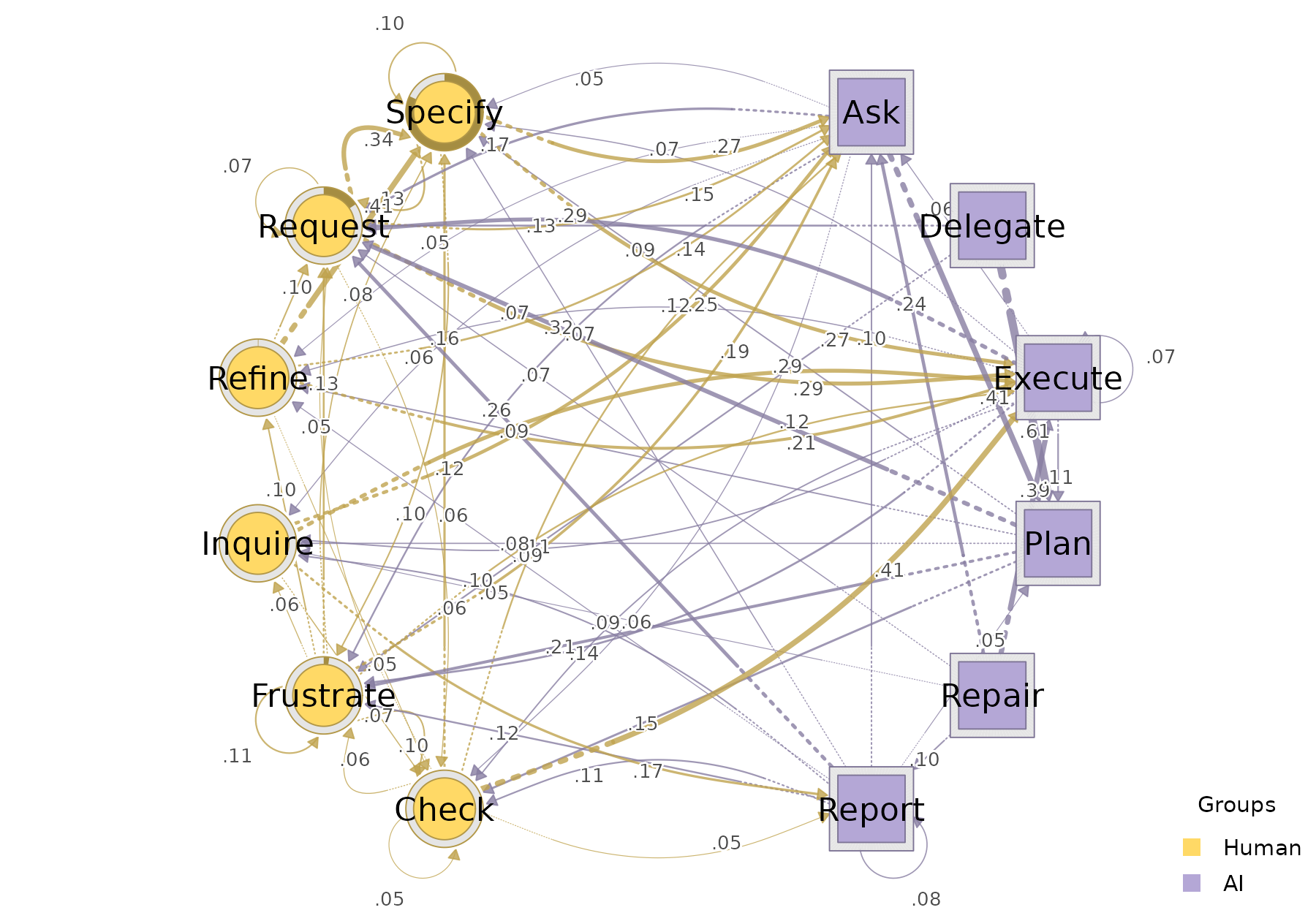

3. Per-actor sequence plots

sequence_plot_htna() shows the temporal structure of the sessions. With by = "state" (the default) each cell is coloured by its code; with by = "group" cells are coloured by actor type. type selects the layout: "index" renders one row per session, "heatmap" collapses across sessions into a single carpet, and "distribution" shows the state composition per timepoint as a stacked area.

sequence_plot_htna(net, by = "state", type = "index")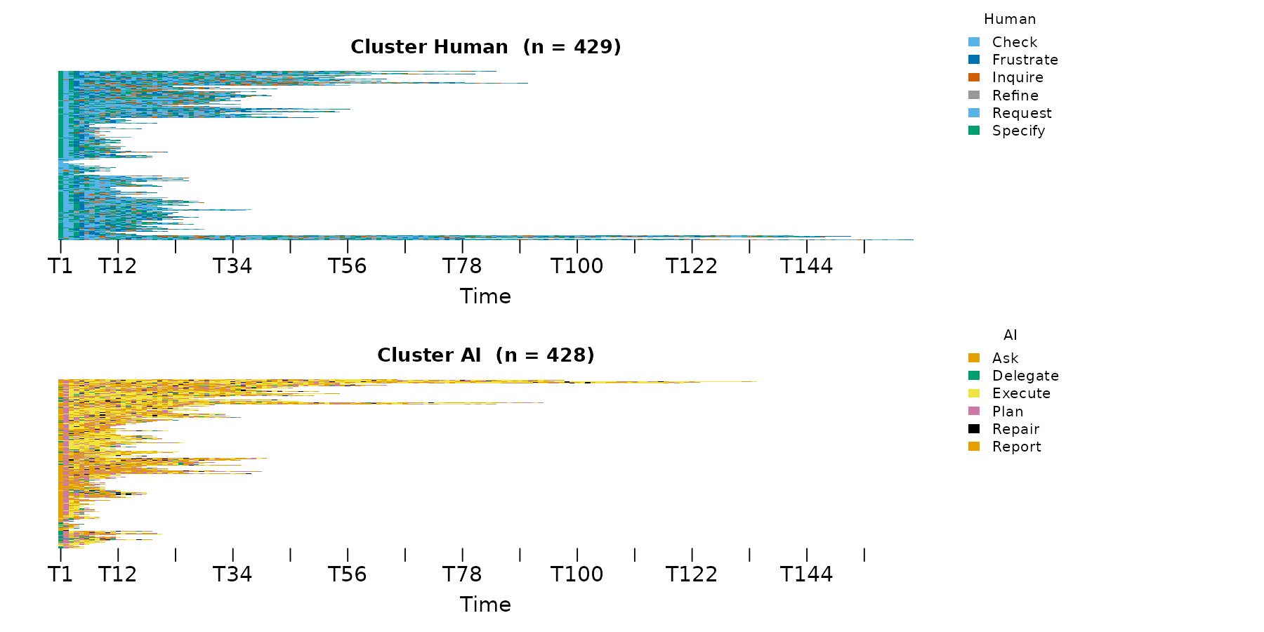

sequence_plot_htna(net, by = "state", type = "heatmap")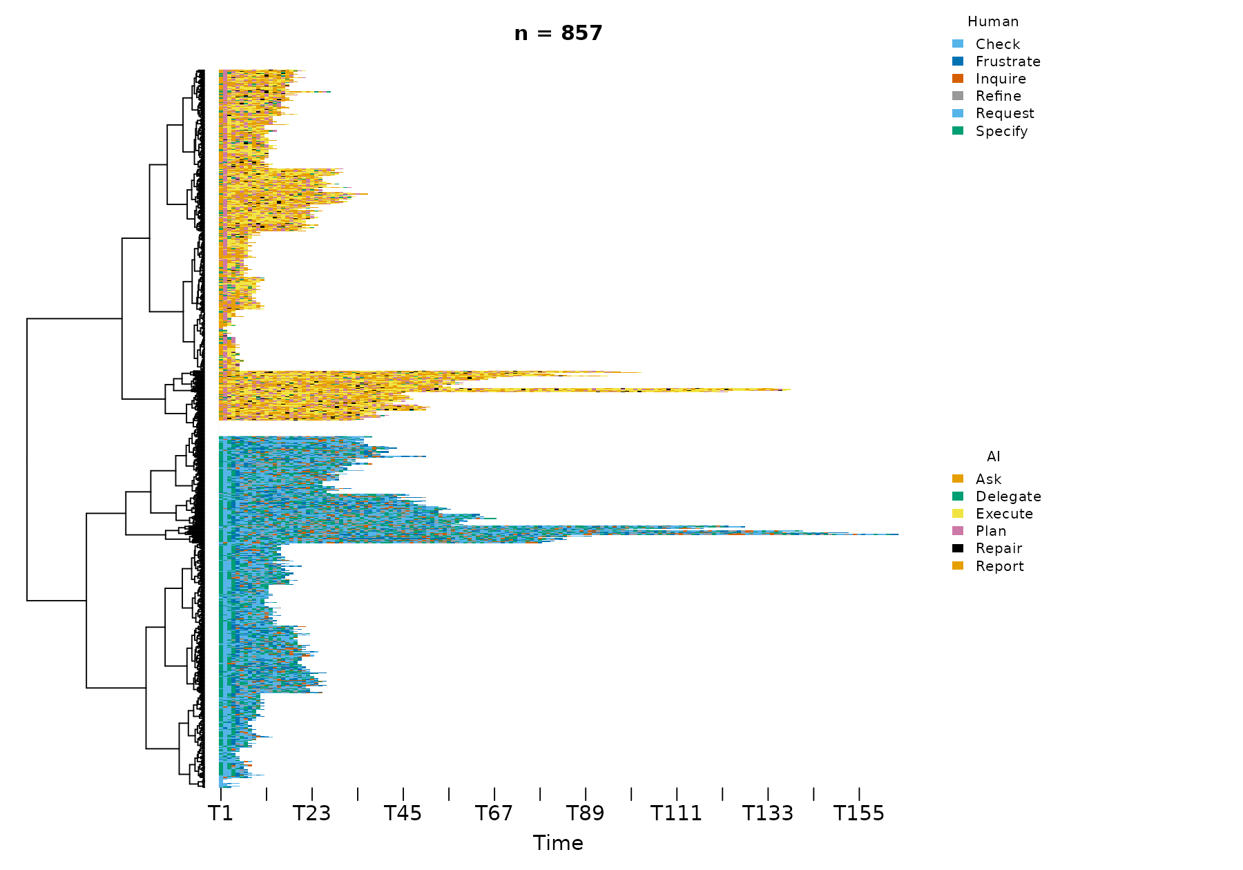

sequence_plot_htna(net, by = "group", type = "distribution", na_color = "white")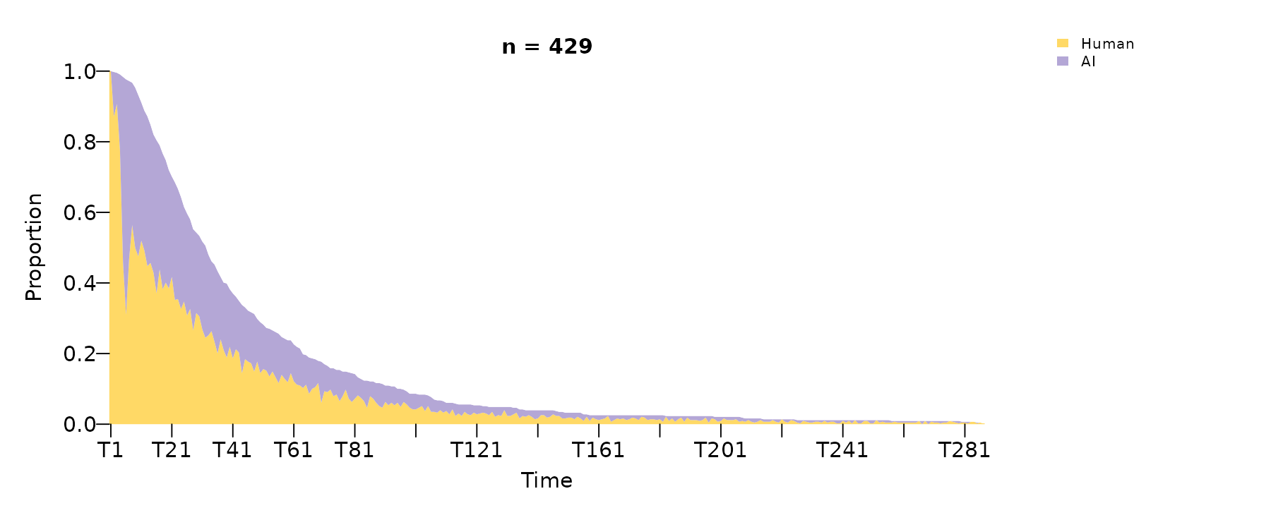

When by = "state", the legend is split into one block per actor type with the actor type name above each block, so the reader can tell at a glance which codes belong to which actor type.

4. Centralities

centralities_htna() returns per-node centrality measures: one row per node, one column per measure, defaulting to nine standard measures (out/in strength, in/out closeness, closeness, betweenness, RSP betweenness, diffusion, clustering). Pass measures = c(...) to restrict to a specific set.

centralities_htna(net)
#>         node actor OutStrength InStrength ClosenessIn ClosenessOut  Closeness
#> 1        Ask    AI   0.9817642  1.5266008 0.012587425  0.006192077 0.01670617
#> 2      Check Human   0.9499230  0.7522288 0.008035193  0.006492281 0.01340661
#> 3   Delegate    AI   1.0000000  0.1740318 0.003015314  0.007567519 0.01315340
#> 4    Execute    AI   0.9256198  2.0338718 0.016720393  0.006367002 0.01784416
#> 5  Frustrate Human   0.8861885  0.9672100 0.010511066  0.006322199 0.01169411
#> 6    Inquire Human   0.9671362  0.5147284 0.006592669  0.007311931 0.01399616
#> 7       Plan    AI   0.9967742  1.2496499 0.012325008  0.006926899 0.01675952
#> 8     Refine Human   1.0000000  0.4703420 0.005943026  0.006143417 0.01250189
#> 9     Repair    AI   0.9960474  0.1995057 0.002655997  0.007958047 0.01404200
#> 10    Report    AI   0.9225146  0.5246300 0.005125410  0.007099789 0.01180054
#> 11   Request Human   0.9329032  1.6926517 0.016089323  0.005980693 0.01812498
#> 12   Specify Human   0.8991424  1.3525625 0.013064153  0.006197358 0.01619607
#>    Betweenness BetweennessRSP Diffusion Clustering
#> 1           13             91  8.778380  0.1543463
#> 2            0             42  8.354335  0.2074548
#> 3            0              3  9.003808  0.1868121
#> 4           29            118  8.186741  0.1359230
#> 5            2             61  7.948727  0.2014196
#> 6           14             27  8.615216  0.1703483
#> 7           25             63  8.715568  0.1531488
#> 8            0             23  8.751161  0.2393259
#> 9            0              1  8.852837  0.2039989
#> 10           0             17  8.186046  0.1557107
#> 11          19            110  8.181829  0.1842378
#> 12          15             88  8.008017  0.2112340

To plot centralities, the plot_centralities() function can be used. Each panel is one measure; bars are coloured per state by default, or by actor type with by = "group":

plot_centralities(net, by = "state")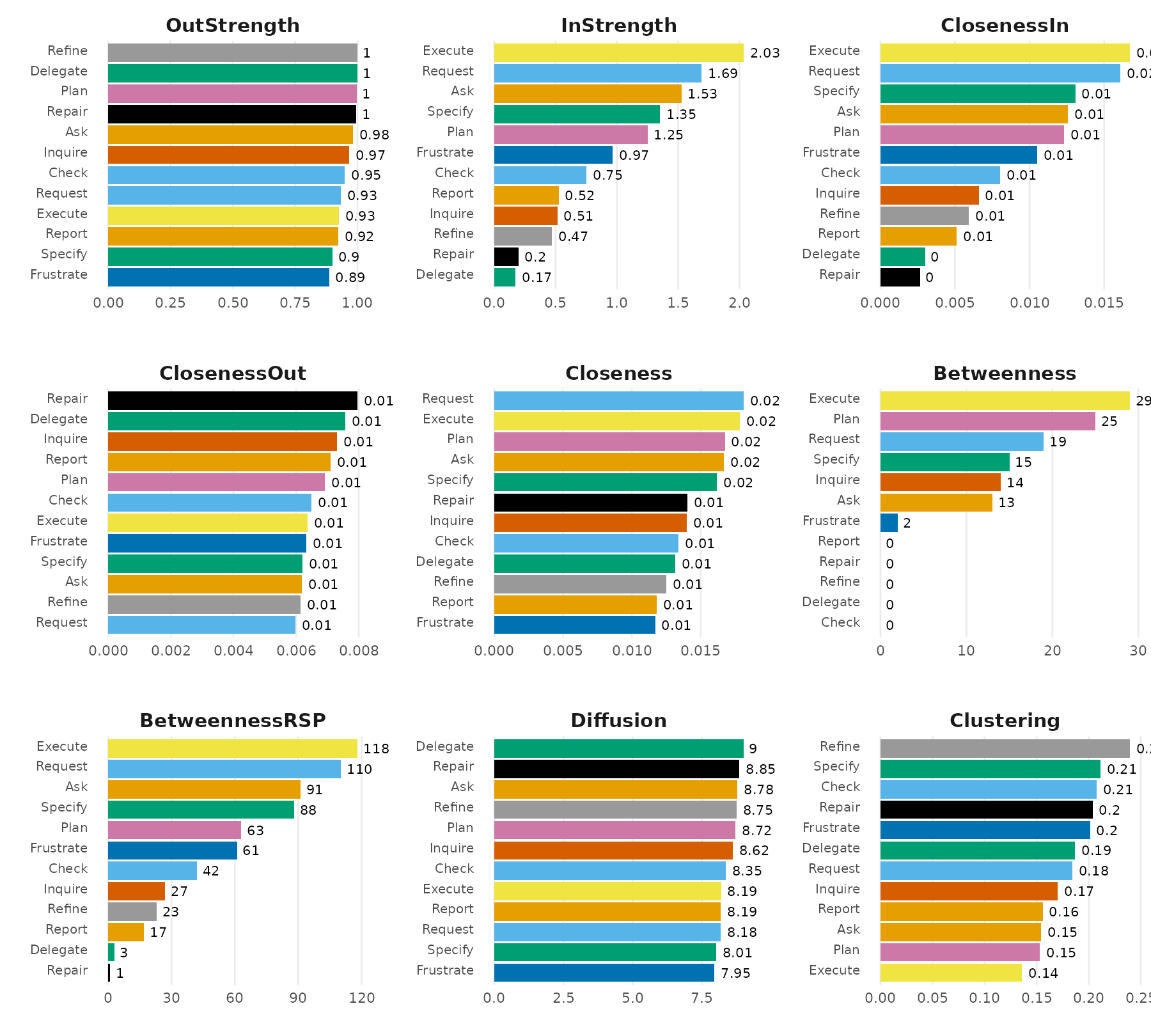

plot_centralities(net, by = "group")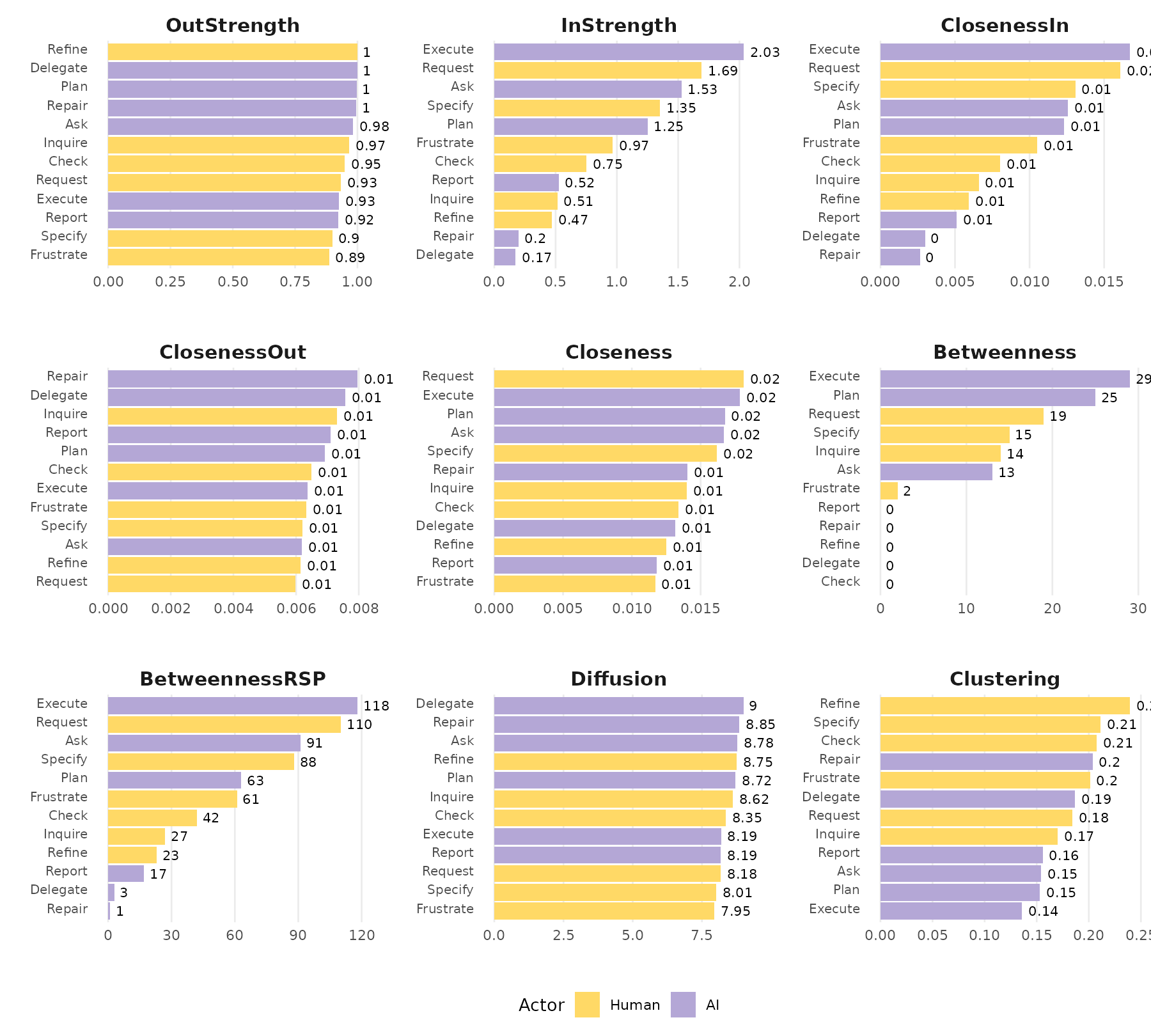

5. Bootstrap

To validate which transitions of an HTNA model are stable, bootstrap_htna() resamples sessions to obtain edge-weight stability and per-edge p-values. plot_htna_bootstrap() renders the resampled network. By default (display = "styled") all edges are shown, with non-significant edges dashed; pass display = "significant" to keep only the edges that pass the significance threshold.

boot <- bootstrap_htna(net)
plot_htna_bootstrap(boot)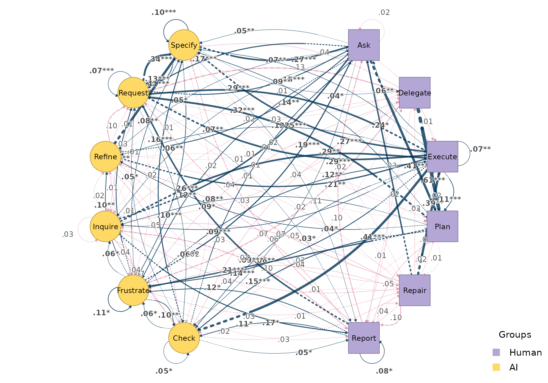

plot_htna_bootstrap(boot, display = "significant")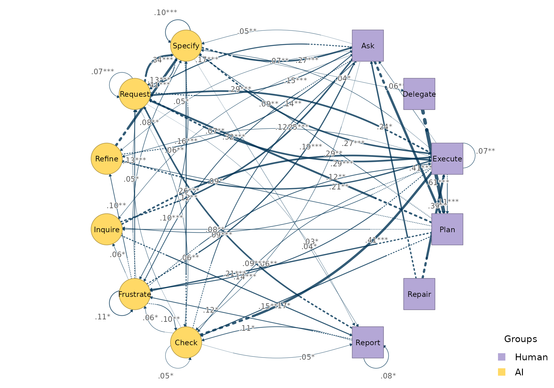

6. Centrality stability

The function centrality_stability_htna() runs a case-dropping centrality stability check: drops a proportion of the sessions, recomputes the centralities, and measures how strongly the dropped-sample centralities correlate with the originals. The returned cs value per measure is the largest drop proportion at which the correlation with the original centralities still meets the threshold (default 0.7) for at least certainty (default 0.95) of resamples — values above ~0.5 are typically considered stable.

cs <- centrality_stability_htna(net, iter = 100, seed = 1)
cs$cs
#>  InStrength OutStrength Betweenness 
#>         0.9         0.9         0.9

By default the check covers InStrength, OutStrength, and Betweenness — the three measures whose values are bit-equal between htna’s cograph engine and the reference implementation.

7. Split-half reliability

The function reliability_htna() reports how stable each edge weight is under random split-half resampling: it draws iter random splits of the sessions, builds a network on each half, and summarises the agreement (mean / median / max absolute deviation, plus correlation) between paired half-networks.

rel <- reliability_htna(net, iter = 100, seed = 1)
rel$summary
#>      model     metric        mean           sd
#> 1 relative   mean_dev 0.012458419 0.0011464861
#> 2 relative median_dev 0.007500373 0.0008826226
#> 3 relative        cor 0.982010309 0.0049162608
#> 4 relative    max_dev 0.098166765 0.0312836964

8. Comparing two networks

Given two HTNA networks built over the same node set, plot_htna_diff() draws the edge-level pairwise difference. Positive differences are green, negative red.

For example, we compare early vs. late sessions using the phase column in the dataset:

grouped <-  build_htna(human_ai, actor_type = "actor_type", group = "phase")

early <- grouped[["Early"]]
late  <- grouped[["Late"]]

plot_htna_diff(early, late)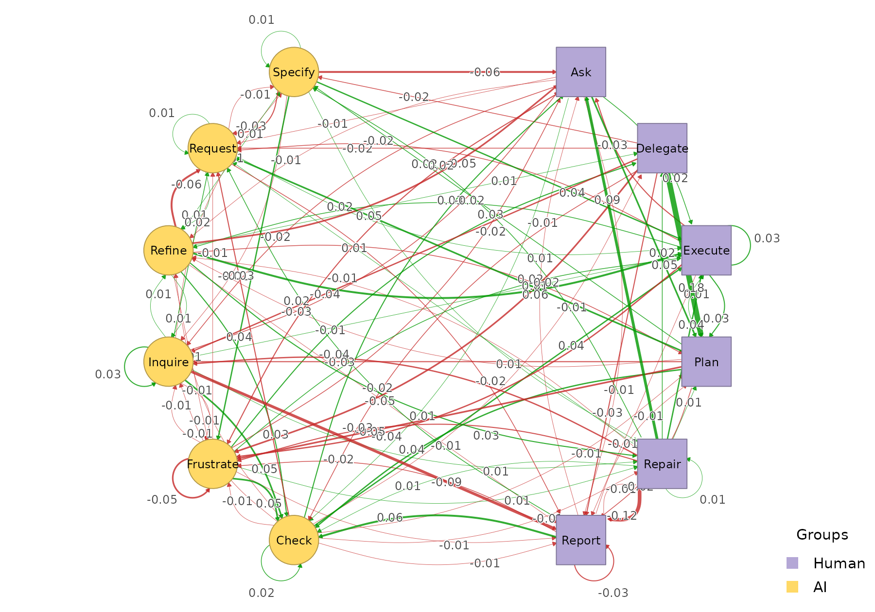

9. Permutation test

The function permutation_htna() provides a non-parametric significance test on each edge weight difference. Pass the result to plot_htna_diff() to render significant differences with the pos/neg colouring above; non-significant edges are dashed grey when show_nonsig = TRUE.

perm <- permutation_htna(early, late, iter = 200)
plot_htna_diff(perm)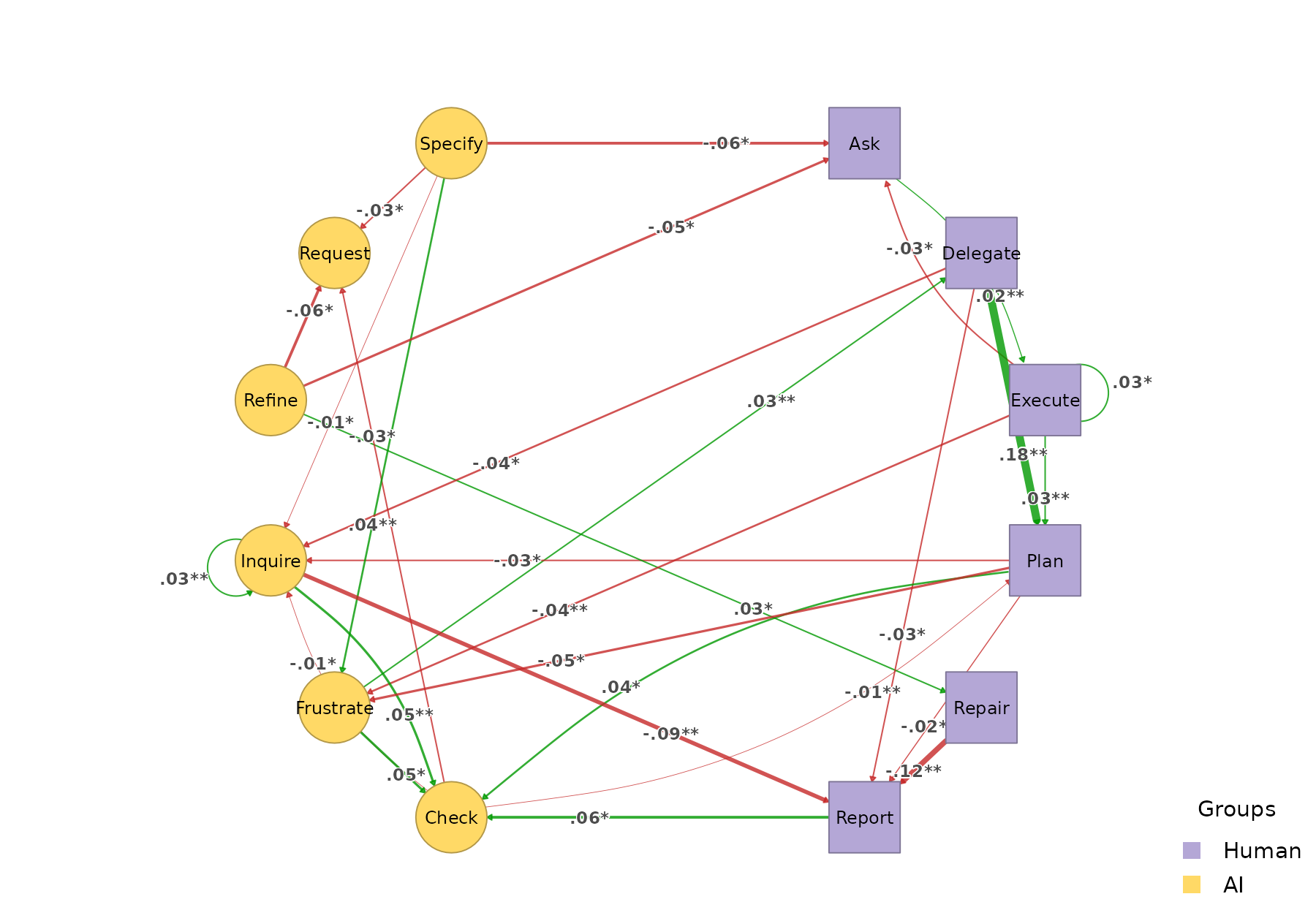

plot_htna_diff(perm, show_nonsig = TRUE)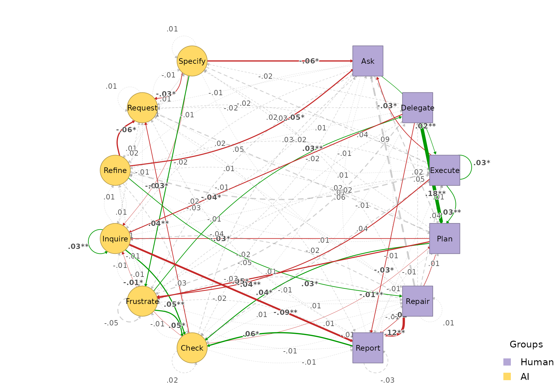

10. Path patterns

extract_meta_paths() discovers recurring patterns at two levels. By default it returns concrete state-level patterns (alphabet = the code set Ask, Plan, Check, …) and annotates each row with the type-level template it instantiates:

extract_meta_paths(net, length = 3)
#> Patterns (state-level) over 429 sequences
#> Rows: 1058 | Lengths: 3 | Gaps: 0
#>                       schema         meta_schema length gap count n_seq support
#>    Request->Execute->Request    Human->AI->Human      3   0   401   194   0.452
#>    Execute->Request->Execute       AI->Human->AI      3   0   391   180   0.420
#>        Request->Specify->Ask    Human->Human->AI      3   0   344   202   0.471
#>           Specify->Ask->Plan       Human->AI->AI      3   0   340   197   0.459
#>           Ask->Plan->Request       AI->AI->Human      3   0   303   197   0.459
#>    Request->Specify->Execute    Human->Human->AI      3   0   281   152   0.354
#>    Execute->Request->Specify    AI->Human->Human      3   0   249   142   0.331
#>  Request->Specify->Frustrate Human->Human->Human      3   0   248   241   0.562
#>         Frustrate->Ask->Plan       Human->AI->AI      3   0   214   187   0.436
#>    Specify->Request->Specify Human->Human->Human      3   0   198   192   0.448
#>  frequency  lift
#>      0.022  5.00
#>      0.021  4.65
#>      0.019  6.15
#>      0.018 11.65
#>      0.016  9.77
#>      0.015  3.73
#>      0.013  3.30
#>      0.013  5.86
#>      0.012 11.71
#>      0.011  2.93
#> ... (1048 more)

A schema filters the search. Each part can be a type name (expands to every code in that group), a concrete state, or *:

extract_meta_paths(net, schema = "Human->AI->Human")
#> State-level instances of schema 'Human->AI->Human' over 429 sequences
#> Rows: 163 | Lengths: 3 | Gaps: 0
#>                       schema      meta_schema length gap count n_seq support
#>    Request->Execute->Request Human->AI->Human      3   0   401   194   0.452
#>    Specify->Execute->Request Human->AI->Human      3   0   176   107   0.249
#>        Request->Ask->Request Human->AI->Human      3   0   130    91   0.212
#>      Check->Execute->Request Human->AI->Human      3   0   123    96   0.224
#>        Specify->Ask->Request Human->AI->Human      3   0   120    84   0.196
#>  Specify->Execute->Frustrate Human->AI->Human      3   0   114    88   0.205
#>  Request->Execute->Frustrate Human->AI->Human      3   0   106    88   0.205
#>    Request->Execute->Inquire Human->AI->Human      3   0    97    76   0.177
#>      Specify->Ask->Frustrate Human->AI->Human      3   0    86    70   0.163
#>    Inquire->Execute->Request Human->AI->Human      3   0    73    52   0.121
#>  frequency lift
#>      0.112 5.00
#>      0.049 2.33
#>      0.036 2.19
#>      0.034 3.67
#>      0.033 2.15
#>      0.032 2.57
#>      0.030 2.24
#>      0.027 4.40
#>      0.024 2.61
#>      0.020 3.31
#> ... (153 more)
extract_meta_paths(net, schema = "Human->Ask->*")
#> State-level instances of schema 'Human->Ask->*' over 429 sequences
#> Rows: 63 | Lengths: 3 | Gaps: 0
#>                   schema      meta_schema length gap count n_seq support
#>       Specify->Ask->Plan    Human->AI->AI      3   0   340   197   0.459
#>     Frustrate->Ask->Plan    Human->AI->AI      3   0   214   187   0.436
#>       Request->Ask->Plan    Human->AI->AI      3   0   139   106   0.247
#>    Request->Ask->Request Human->AI->Human      3   0   130    91   0.212
#>    Specify->Ask->Request Human->AI->Human      3   0   120    84   0.196
#>  Specify->Ask->Frustrate Human->AI->Human      3   0    86    70   0.163
#>       Inquire->Ask->Plan    Human->AI->AI      3   0    53    45   0.105
#>        Refine->Ask->Plan    Human->AI->AI      3   0    52    46   0.107
#>  Request->Ask->Frustrate Human->AI->Human      3   0    50    44   0.103
#>    Specify->Ask->Specify Human->AI->Human      3   0    49    41   0.096
#>  frequency  lift
#>      0.170 11.65
#>      0.107 11.71
#>      0.070  4.48
#>      0.065  2.19
#>      0.060  2.15
#>      0.043  2.61
#>      0.027  6.22
#>      0.026  6.57
#>      0.025  1.43
#>      0.025  0.93
#> ... (53 more)

Filter by lift to surface over-represented patterns (lift > 1 means more frequent than independence would predict):

extract_meta_paths(net, length = 3, min_lift = 2)
#> Patterns (state-level) over 429 sequences
#> Rows: 301 | Lengths: 3 | Gaps: 0
#>                       schema         meta_schema length gap count n_seq support
#>    Request->Execute->Request    Human->AI->Human      3   0   401   194   0.452
#>    Execute->Request->Execute       AI->Human->AI      3   0   391   180   0.420
#>        Request->Specify->Ask    Human->Human->AI      3   0   344   202   0.471
#>           Specify->Ask->Plan       Human->AI->AI      3   0   340   197   0.459
#>           Ask->Plan->Request       AI->AI->Human      3   0   303   197   0.459
#>    Request->Specify->Execute    Human->Human->AI      3   0   281   152   0.354
#>    Execute->Request->Specify    AI->Human->Human      3   0   249   142   0.331
#>  Request->Specify->Frustrate Human->Human->Human      3   0   248   241   0.562
#>         Frustrate->Ask->Plan       Human->AI->AI      3   0   214   187   0.436
#>    Specify->Request->Specify Human->Human->Human      3   0   198   192   0.448
#>  frequency  lift
#>      0.022  5.00
#>      0.021  4.65
#>      0.019  6.15
#>      0.018 11.65
#>      0.016  9.77
#>      0.015  3.73
#>      0.013  3.30
#>      0.013  5.86
#>      0.012 11.71
#>      0.011  2.93
#> ... (291 more)
extract_meta_paths(net, level = "type", length = 3, min_lift = 1.2)
#> Meta-paths (type-level) over 429 sequences
#> Rows: 3 | Lengths: 3 | Gaps: 0
#>            schema length gap count n_seq support frequency lift
#>  Human->AI->Human      3   0  3593   402   0.937     0.194 1.41
#>  Human->Human->AI      3   0  3172   422   0.984     0.172 1.25
#>     AI->Human->AI      3   0  2744   383   0.893     0.148 1.36