
build_htna() accepts clustering results from the
Nestimate ecosystem as first-class inputs. You can hand a
clustering object straight to build_htna() and get back an
htna-aware result with the actor partition already
attached.
The clustering constructors covered here all operate at the
cohort level: sessions are grouped into k
clusters and one htna network is built per cluster. The result is an
htna_group, identical in shape to what
build_htna(..., group = ...) returns, so every grouped-htna
wrapper (plot_htna(), plot_htna_diff(),
permutation_htna(),
centrality_stability_htna(), etc.) works unchanged.
Setup
library(htna)
data(human_ai)

net <- build_htna(human_ai, actor_type = "actor_type")
Nestimate::build_clusters() (distance-based)
build_clusters() computes a pairwise dissimilarity
between sessions (Hamming by default) and applies a partitioning
algorithm (pam by default) to split them into k
cohorts. Feed the returned net_clustering object straight
to build_htna():
cc  <- Nestimate::build_clusters(net, k = 2, seed = 1)
grp <- build_htna(cc)

class(grp)
#> [1] "htna_group"      "netobject_group" "list"
names(grp)
#> [1] "Cluster 1" "Cluster 2"
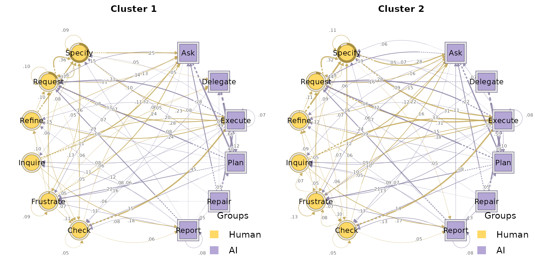
The result is an htna_group: one htna network per
cluster, each carrying the same actor partition inherited from
net. Plot the two cohorts side by side:
par(op)Because both networks share the alphabet, they compose with the comparison wrappers:
plot_htna_diff(grp[[1]], grp[[2]])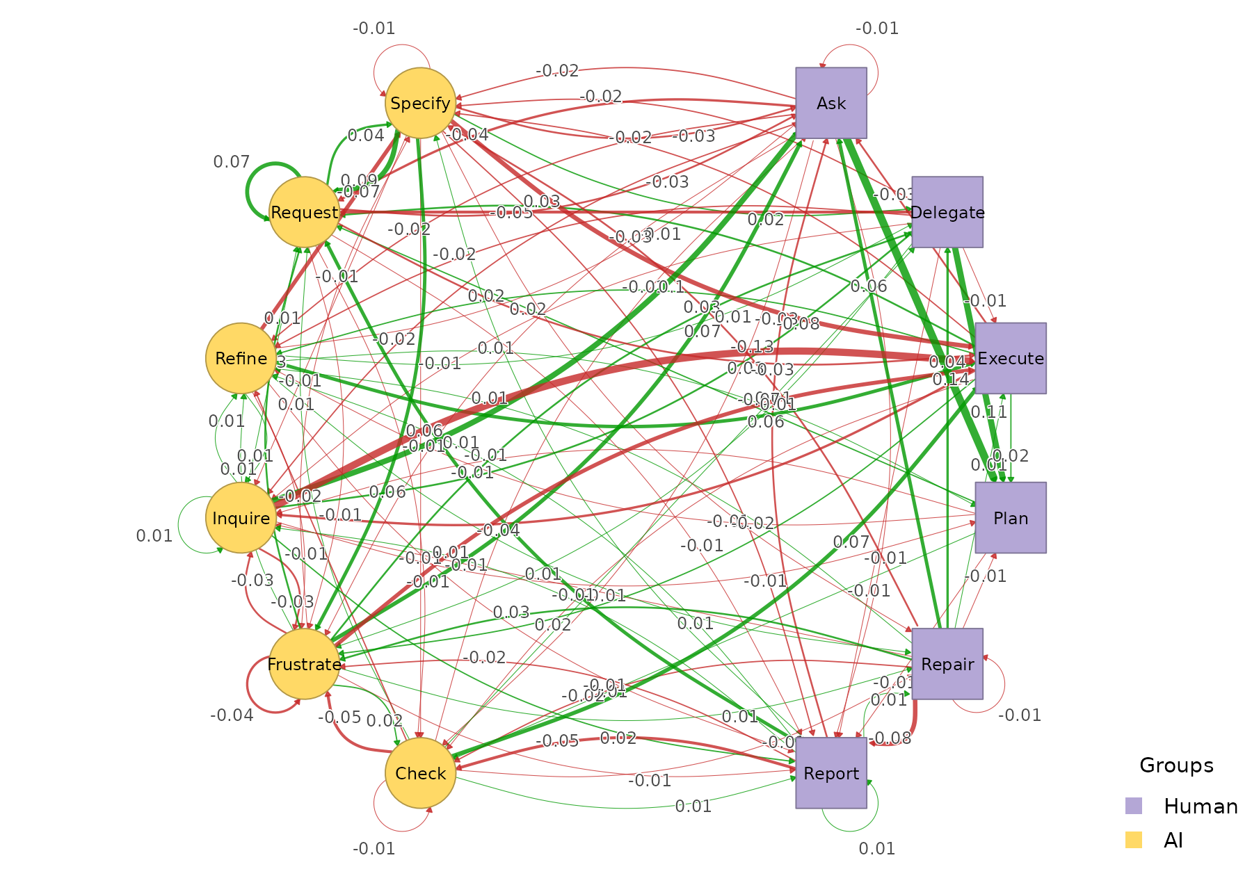
Nestimate::cluster_mmm() (mixture of Markov
chains)
cluster_mmm() fits a k-component mixture of
first-order Markov chains via EM and assigns each session
probabilistically to a component. The returned net_mmm
object is also a legal build_htna() input:
cm    <- Nestimate::cluster_mmm(net, k = 2, seed = 1)
grp_m <- build_htna(cm)

names(grp_m)
#> [1] "Cluster 1" "Cluster 2"
grp_m is again an htna_group, ready to feed
any of the grouped wrappers.
build_clusters() and cluster_mmm() answer
different questions: build_clusters() groups sessions by
trajectory similarity under a fixed distance metric;
cluster_mmm() groups sessions by the first-order transition
process most likely to have generated them. The Nestimate documentation
covers the trade-offs.
Choosing the number of clusters
Both constructors take a k. Two Nestimate helpers sweep a range of candidate values and score them, so the choice does not have to be made blind. A third helper reports per-cluster quality once a particular fit has been settled on.
For build_clusters():
cluster_choice()
cluster_choice() fits the same partitioning algorithm at
each k in a grid and reports the average silhouette width, mean
within-cluster distance, and the cluster-size range. Higher silhouette
(closer to 1) is better; extreme size ratios flag partitions with a
single dominant cluster and a tiny satellite. The row flagged
<-- best in the print method is the largest silhouette
across the grid.
Nestimate::cluster_choice(net, k = 2:4)
#> Cluster Choice (sweep: k)
#>
#>  k silhouette within_dist sizes     ratio  best
#>  2 0.756      56.274      [11, 418] 38.000 <-- best
#>  3 0.501      49.323      [11, 349] 31.727
#>  4 0.503      48.827      [5, 349]  69.800
For cluster_mmm(): compare_mmm()
compare_mmm() fits the mixture at each candidate
k and returns the standard information criteria
(AIC, BIC, ICL) plus the average
posterior probability (AvePP, higher = more confident
assignments) and normalised entropy (lower = more separated components).
The row flagged <-- BIC is the best BIC across the grid;
ICL trades off fit against classification uncertainty and is often
preferred when the cohorts must be used for downstream inference.
Nestimate::compare_mmm(net, k = 2:3, seed = 1)
#> MMM Model Comparison
#>
#>  k log_likelihood AIC      BIC      ICL      AvePP     Entropy   converged
#>  2 -36345.27      73264.54 74430.17 74510.27 0.9211857 0.2658902 TRUE
#>  3 -36115.29      73092.59 74843.08 74932.82 0.9136712 0.1967376 TRUE
#>  best
#>  <-- BIC
#>
Validating a specific fit: cluster_diagnostics()
Once you have picked a k and fit the clustering, pass the
result to cluster_diagnostics() to see per-cluster sizes,
mean within- cluster distance, and silhouette. Small satellites or
negative silhouettes on one cluster indicate that the partition is
stretched by outliers even if the aggregate score is acceptable.
Nestimate::cluster_diagnostics(cc)
#> Cluster Diagnostics (distance) [pam / hamming]
#>   Sequences: 429  |  Clusters: 2
#>   Quality: silhouette = 0.300
#>
#>   Cluster  N            Mean within-dist  Silhouette
#>   1        288 (67.1%)  36.300            0.552
#>   2        141 (32.9%)  93.620            -0.215
Comparing the resulting cohorts
Once clustering has produced an htna_group,
compare_htna() computes a descriptive summary of every
cohort pair in one call — you do not need to pull out individual cohorts
by hand.
comparisons <- compare_htna(grp)

class(comparisons)
#> [1] "htna_comparison_group" "list"
names(comparisons)
#> [1] "Cluster 1 vs Cluster 2"
Each element is an htna_comparison: the
Nestimate net_comparison fields
(summary_metrics, edge_metrics,
network_metrics, matrices,
difference_matrix) plus an htna-aware
actor_pair_metrics table that summarises the difference for
every directed actor-type block:
one <- comparisons[[1]]
one$summary_metrics
#>                category               metric       value
#> 1     Weight Deviations      Mean Abs. Diff.  0.02025425
#> 2     Weight Deviations    Median Abs. Diff.  0.01020158
#> 3     Weight Deviations            RMS Diff.  0.03290003
#> 4     Weight Deviations       Max Abs. Diff.  0.14058447
#> 5     Weight Deviations Rel. Mean Abs. Diff.  0.24305095
#> 6     Weight Deviations             CV Ratio  1.09485122
#> 7          Correlations              Pearson  0.95470530
#> 8          Correlations             Spearman  0.94189862
#> 9          Correlations              Kendall  0.80856141
#> 10         Correlations             Distance  0.88970520
#> 11      Dissimilarities            Euclidean  0.39480036
#> 12      Dissimilarities            Manhattan  2.91661145
#> 13      Dissimilarities             Canberra 23.14861488
#> 14      Dissimilarities          Bray-Curtis  0.12152548
#> 15      Dissimilarities            Frobenius  0.16117657
#> 16         Similarities               Cosine  0.97133126
#> 17         Similarities              Jaccard  0.78328539
#> 18         Similarities                 Dice  0.87847452
#> 19         Similarities              Overlap  0.87847452
#> 20         Similarities                   RV  0.95884110
#> 21 Pattern Similarities       Rank Agreement  0.88636364
#> 22 Pattern Similarities       Sign Agreement  0.97916667
head(one$actor_pair_metrics)
#>   source_actor target_actor n_cells n_nonzero_x n_nonzero_y n_changed
#> 1        Human        Human      36          35          35        35
#> 2        Human           AI      36          36          36        36
#> 3           AI        Human      36          34          36        36
#> 4           AI           AI      36          27          28        28
#>   mean_difference mean_absolute_difference rms_difference
#> 1     0.001072078               0.01887634     0.02928339
#> 2    -0.001072078               0.02612978     0.04044685
#> 3    -0.005198687               0.01894510     0.02313669
#> 4     0.005198687               0.01706576     0.03606767
#>   max_absolute_difference
#> 1              0.09083051
#> 2              0.13076689
#> 3              0.05596170
#> 4              0.14058447
plot() dispatches through
plot.htna_comparison_group() and draws one panel per pair
with the actor styling preserved:
plot(comparisons)For a full statistical test of the same pairs, feed the group to
permutation_htna() instead — see the grouped vignette.