State frequencies and chi-square mosaics

In this vignette, we look at additional summary functions and visualizations in htna. We will use two networks constructed from the bundled human_ai corpus (Human + AI events tagged by actor_type; see ?human_ai). The frequency family operates on either, but the mosaic family requires an integer-weighted network because the chi-square test acts on counts; this is the network produced under method = "frequency".

library(htna)
data(human_ai)

net      <- build_htna(human_ai, actor_type = "actor_type")
net_freq <- build_htna(human_ai, actor_type = "actor_type",
                       method = "frequency")

Marginal state distributions

Tabular summary

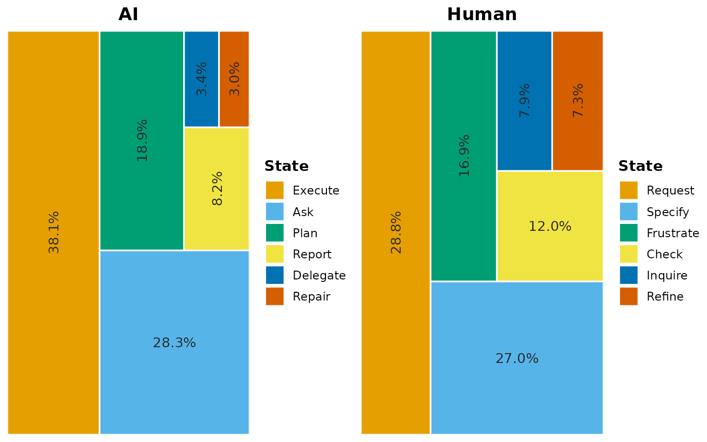
frequencies_htna() returns the per-actor marginal state distribution as a data frame with one row per (actor_type, state) pair. Columns are: actor type (group), state, count, and within-network proportion. The table is the data underlying every chart in this section.

frequencies_htna(net)
#>    group     state count proportion
#> 1     AI   Execute  3258 0.38100807
#> 2  Human   Request  3104 0.28751389
#> 3  Human   Specify  2920 0.27047054
#> 4     AI       Ask  2416 0.28254005
#> 5  Human Frustrate  1829 0.16941460
#> 6     AI      Plan  1620 0.18945153
#> 7  Human     Check  1298 0.12022971
#> 8  Human   Inquire   853 0.07901074
#> 9  Human    Refine   792 0.07336050
#> 10    AI    Report   705 0.08244650
#> 11    AI  Delegate   295 0.03449889
#> 12    AI    Repair   257 0.03005496

Graphical summary: plot_frequencies_htna()

plot_frequencies_htna() renders the same marginal distribution in three layouts. Each layout encodes the same data but is optimised for a different reading task.

Treemap (view = "treemap", default)

Each panel corresponds to one actor; tile area within a panel encodes the within-network proportion of the corresponding state. The layout is space-efficient and allows the full state vocabulary to be displayed simultaneously.

plot_frequencies_htna(net)

Combined bars (view = "bars")

The bars layout collapses both actor types onto a single y-axis, sorts the states by total count, and colours the bars by actor. This layout is appropriate when the analytic task is direct numerical comparison across the full vocabulary.

plot_frequencies_htna(net, view = "bars")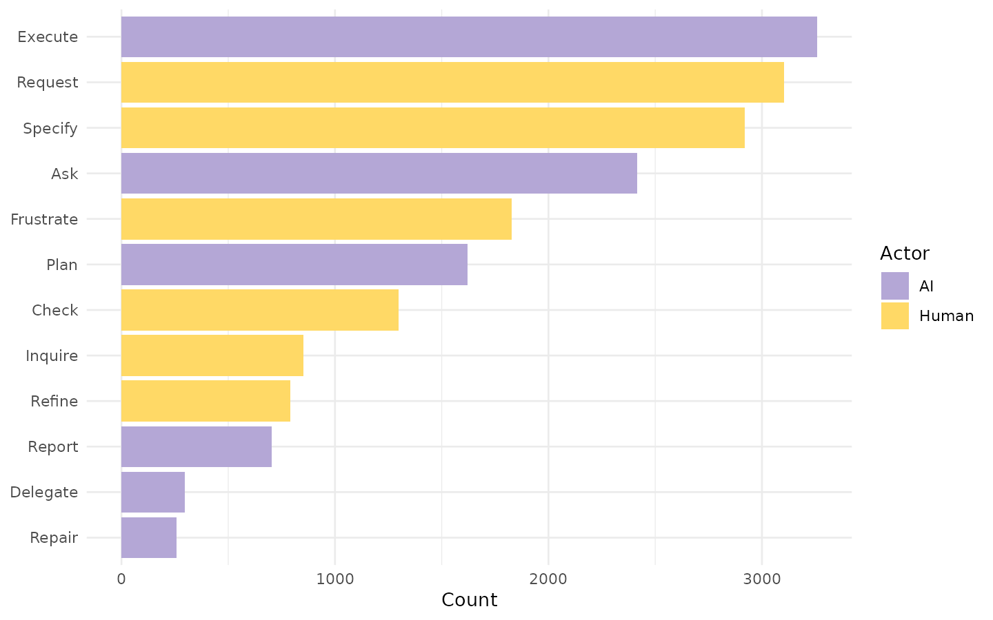

The bars layout returns a ggplot object, permitting modification through standard ggplot composition operators:

plot_frequencies_htna(net, view = "bars") +
  ggplot2::labs(title = "Human vs AI: state counts")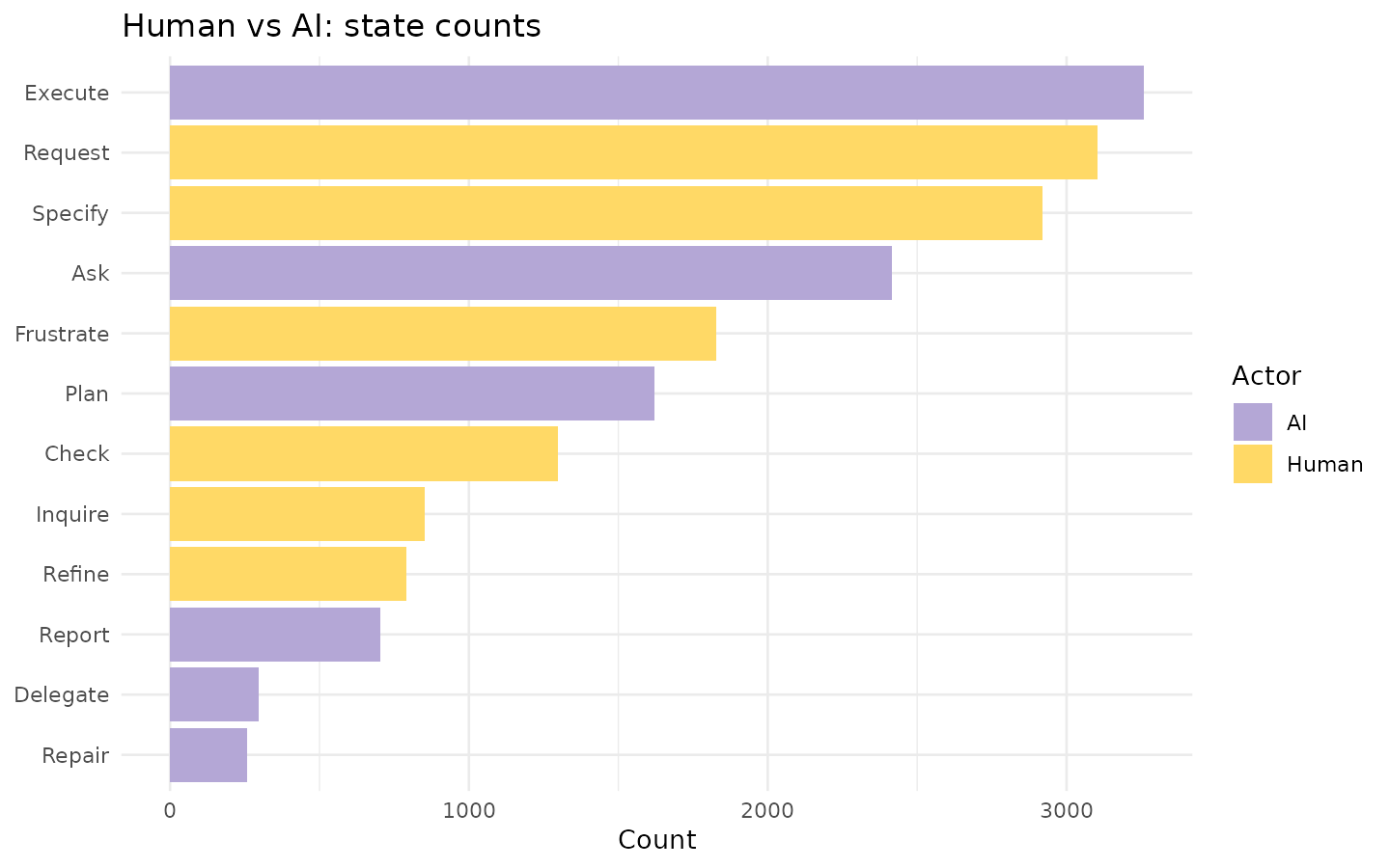

Per-actor faceted bars (view = "facet")

The faceted layout assigns each actor its own panel with an independent y-axis. This is appropriate when the actors differ substantially in event volume, since a shared scale would compress the lower-volume actor’s bars beyond legibility.

plot_frequencies_htna(net, view = "facet")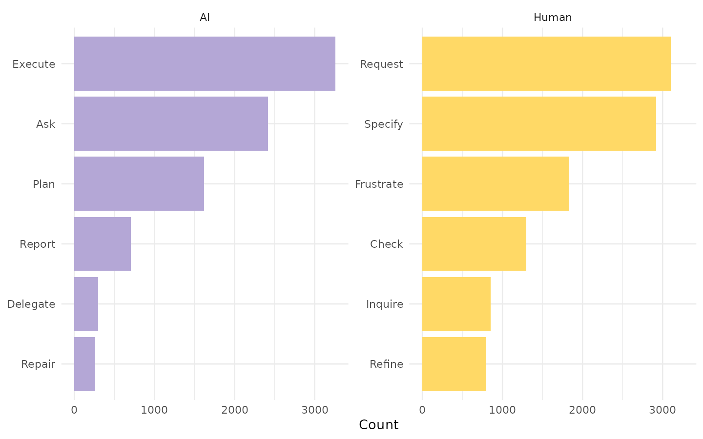

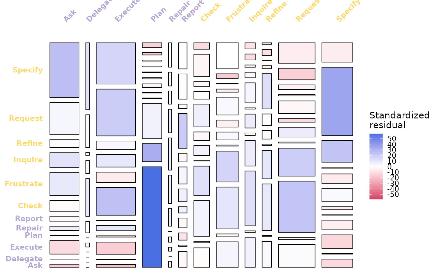
Joint transition distribution: chi-square mosaic

mosaic_plot_htna() displays the joint distribution of (source, target) transitions as a chi-square mosaic. Each cell of the transition matrix is rendered as a rectangle whose area is proportional to the joint share of that transition; cell colour encodes the standardised residual against an independence model. Cells with positive residuals (over-represented relative to independence) are coloured blue; cells with negative residuals (under-represented) are coloured red; cells whose observed value matches the independence prediction are white.

The chi-square test requires integer counts, hence the requirement for a frequency-method network.

Default residuals (permutation-based)

The default residual estimator is permutation-based, with n_perm = 500 iterations. Permutation residuals are appropriate when cell counts are sparse or when the chi-square asymptotic approximation is not trusted; the trade-off is computation time.

mosaic_plot_htna(net_freq, seed = 1L)

Cells with strong positive residuals identify transitions that characterise the process beyond what would be expected by chance; cells with strong negative residuals identify transitions that are systematically suppressed.

Asymptotic residuals (residuals = "asymptotic")

The closed-form chi-square standardised residual estimator (chisq.test()$stdres) is faster and is the convention used by tna and vcd. It is appropriate when cell counts are large enough for the asymptotic approximation to hold.

mosaic_plot_htna(net_freq, residuals = "asymptotic")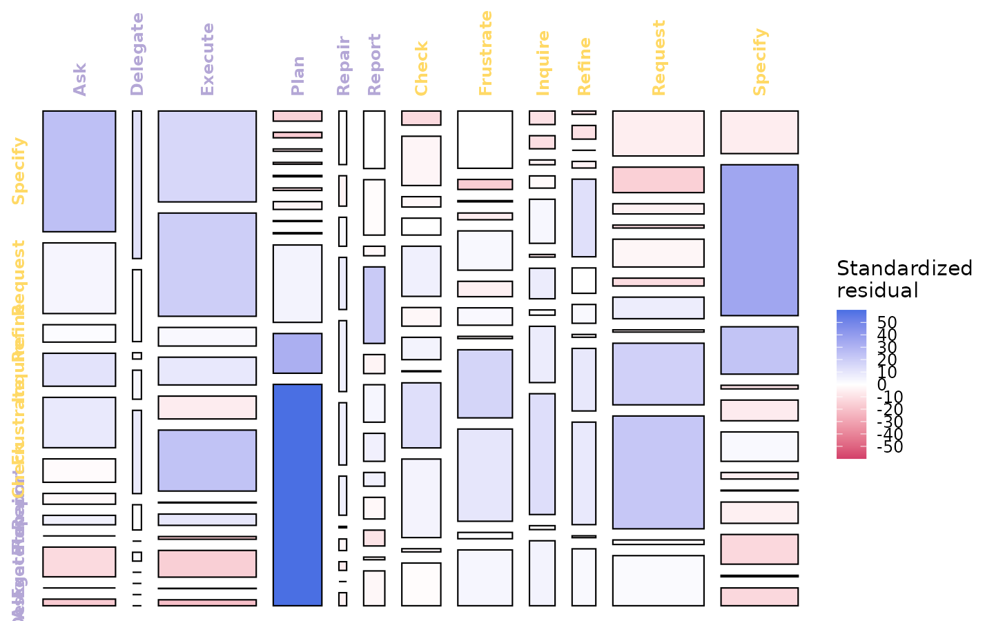

For htna corpora of typical size (hundreds of sessions, hundreds to thousands of transitions per cell), permutation and asymptotic residuals agree closely.

Colour-scale clipping (range = c(-4, 4))

By default the colour scale is calibrated to the maximum absolute residual in the matrix. A single extreme cell can therefore desaturate the remainder of the chart. Clipping the range to a fixed interval preserves contrast across the matrix and supports comparison of mosaics across networks.

mosaic_plot_htna(net_freq, range = c(-4, 4), seed = 1L)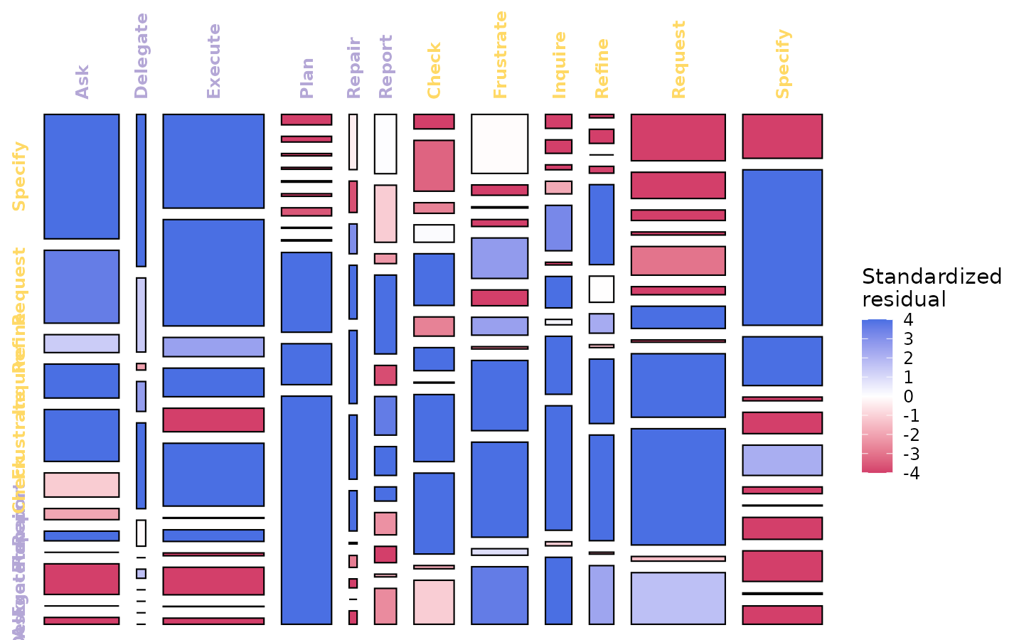

A range of ±4 is conventional in mosaic displays; residuals beyond the range saturate to the most intense colour.

Axis-label rotation (top_angle, left_angle)

For matrices with long state names or large vocabularies, axis labels may collide. The top_angle and left_angle arguments rotate the labels for legibility.

mosaic_plot_htna(net_freq, top_angle = 45, left_angle = 0, seed = 1L)