This vignette showcases some basic usage of the tna
package. For more tutorials, please visit the package website.
First we load the package that we will use for this example.
We also load the group_regulation data available in the
package (see ?group_regulation for further information)
data("group_regulation", package = "tna")We build a TNA model using this data with the tna()
function .
tna_model <- tna(group_regulation)To visualize the model, we can use the standard plot()
function.
plot(tna_model)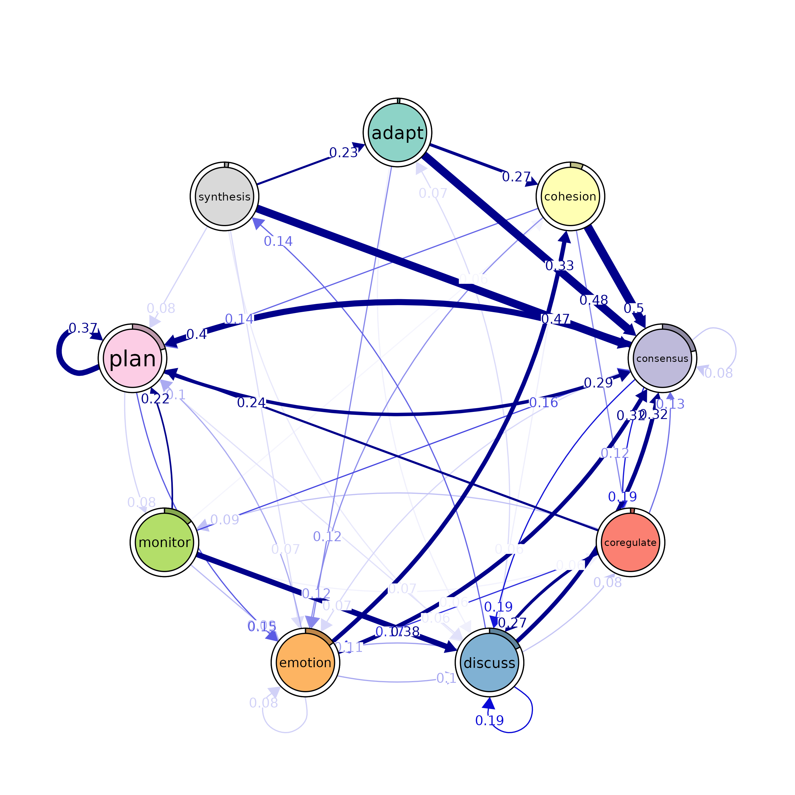
The initial state probabilities are
data.frame(`Initial prob.` = tna_model$inits, check.names = FALSE) |>
  rownames_to_column("Action") |>
  arrange(desc(`Initial prob.`)) |>
  gt() |>
fmt_percent()| Action | Initial prob. |
|---|---|
| consensus | 21.40% |
| plan | 20.45% |
| discuss | 17.55% |
| emotion | 15.15% |
| monitor | 14.40% |
| cohesion | 6.05% |
| synthesis | 1.95% |
| coregulate | 1.90% |
| adapt | 1.15% |
and the transitions probabilities are
tna_model$weights |>
  data.frame() |>
  rownames_to_column("From\\To") |>
  gt() |>
fmt_percent()| From\To | adapt | cohesion | consensus | coregulate | discuss | emotion | monitor | plan | synthesis |
|---|---|---|---|---|---|---|---|---|---|
| adapt | 0.00% | 27.31% | 47.74% | 2.16% | 5.89% | 11.98% | 3.34% | 1.57% | 0.00% |
| cohesion | 0.29% | 2.71% | 49.79% | 11.92% | 5.96% | 11.56% | 3.30% | 14.10% | 0.35% |
| consensus | 0.47% | 1.49% | 8.20% | 18.77% | 18.80% | 7.27% | 4.66% | 39.58% | 0.76% |
| coregulate | 1.62% | 3.60% | 13.45% | 2.34% | 27.36% | 17.21% | 8.63% | 23.91% | 1.88% |
| discuss | 7.14% | 4.76% | 32.12% | 8.43% | 19.49% | 10.58% | 2.23% | 1.16% | 14.10% |
| emotion | 0.25% | 32.53% | 32.04% | 3.42% | 10.19% | 7.68% | 3.63% | 9.98% | 0.28% |
| monitor | 1.12% | 5.58% | 15.91% | 5.79% | 37.54% | 9.07% | 1.81% | 21.56% | 1.61% |
| plan | 0.10% | 2.52% | 29.04% | 1.72% | 6.79% | 14.68% | 7.55% | 37.42% | 0.18% |
| synthesis | 23.47% | 3.37% | 46.63% | 4.45% | 6.29% | 7.06% | 1.23% | 7.52% | 0.00% |
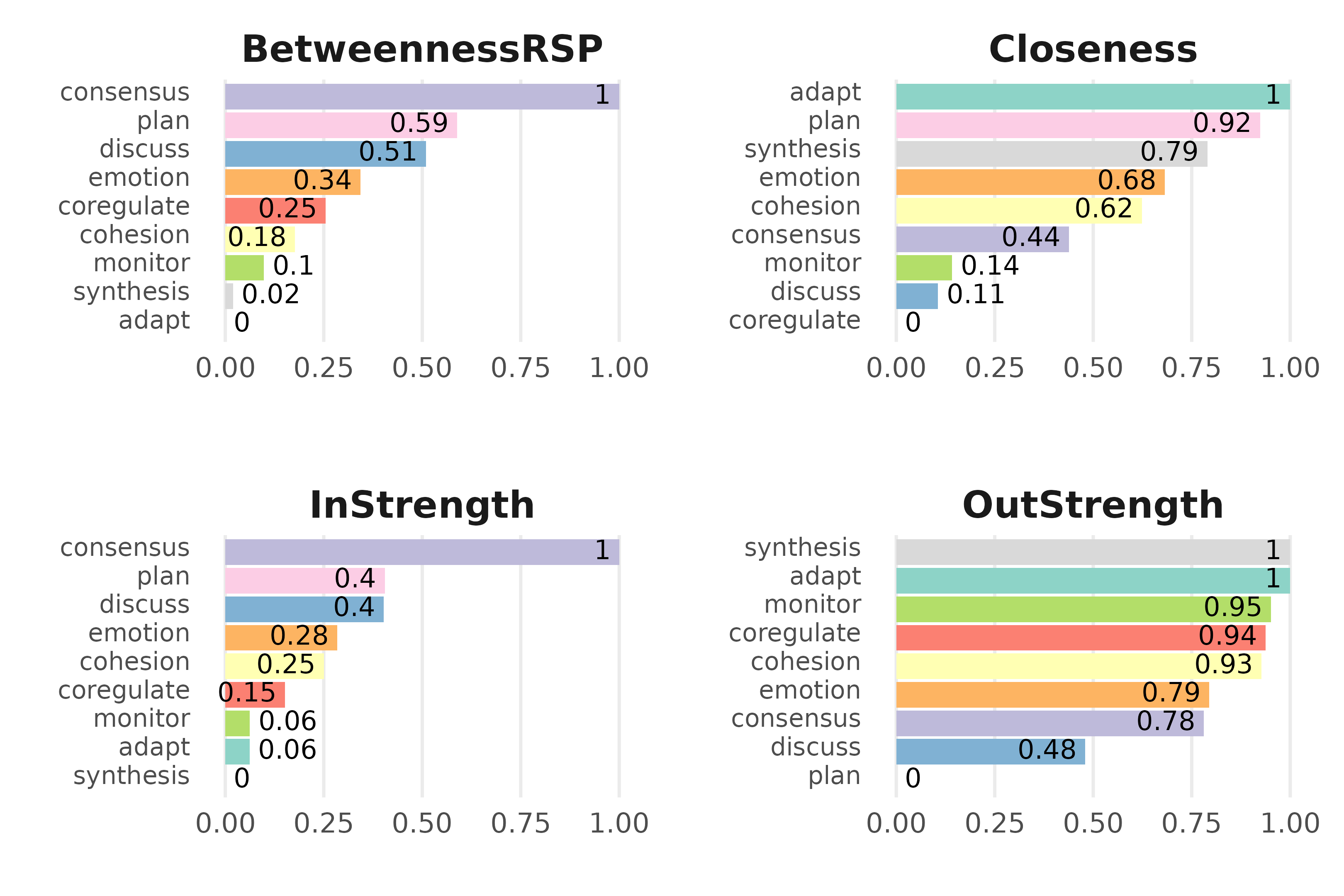
The function centralities() can be used to compute
various centrality measures (see ?centralities for more
information). These measures can also be visualized with the
plot() function.
centrality_measures <- c("BetweennessRSP", "Closeness", "InStrength", "OutStrength")
cents_withoutloops <- centralities(
  tna_model,
  measures = centrality_measures,
  loops = FALSE,
  normalize = TRUE
)
plot(cents_withoutloops, ncol = 2, model = tna_model)