Using grouped sequence data with tna

TNA also enables the analysis of transition networks constructed from grouped sequence data. In this example, we first fit a mixed Markov model to the engagement data using the seqHMM package and build a grouped TNA model based on this model. First, we load the packages we will use for this example.

library("tna")
library("tibble")
library("dplyr")
library("gt")
library("seqHMM")
data("engagement", package = "tna")

We simulate transition probabilities to initialize the model.

set.seed(265)
tna_model <- tna(engagement)
n_var <- length(tna_model$labels)
n_clusters <- 3
trans_probs <- simulate_transition_probs(n_var, n_clusters)
init_probs <- list(
  c(0.70, 0.20, 0.10),
  c(0.15, 0.70, 0.15),
  c(0.10, 0.20, 0.70)
)

Next, we building and fit the model (this step takes some time to compute, the final model object is also available in the tna package as engagement_mmm).

mmm <- build_mmm(
  engagement,
  transition_probs = trans_probs,
  initial_probs = init_probs
)
fit_mmm <- fit_model(
  modelTrans,
  global_step = TRUE,
  control_global = list(algorithm = "NLOPT_GD_STOGO_RAND"),
  local_step = TRUE,
  threads = 60,
  control_em = list(restart = list(times = 100, n_optimum = 101))
)

Now, we create a new model using the cluster information from the model. Alternatively, if sequence data is provided to group_model(), the group assignments can be provided with the group argument.

tna_model_clus <- group_model(fit_mmm$model)

We can summarize the cluster-specific models

summary(tna_model_clus) |>
  gt() |>
  fmt_number(decimals = 2)

metric	Cluster 1	Cluster 2	Cluster 3
Node Count	3.00	3.00	3.00
Edge Count	8.00	9.00	9.00
Network Density	1.00	1.00	1.00
Mean Distance	0.29	0.30	0.27
Mean Out-Strength	1.00	1.00	1.00
SD Out-Strength	0.63	0.69	0.58
Mean In-Strength	1.00	1.00	1.00
SD In-Strength	0.00	0.00	0.00
Mean Out-Degree	2.67	3.00	3.00
SD Out-Degree	0.58	0.00	0.00
Centralization (Out-Degree)	0.25	0.00	0.00
Centralization (In-Degree)	0.25	0.00	0.00
Reciprocity	0.80	1.00	1.00

and their initial probabilities

bind_rows(lapply(tna_model_clus, \(x) x$inits), .id = "Cluster") |>
  gt() |>
  fmt_percent()

Cluster	Active	Average	Disengaged
Cluster 1	75.00%	0.00%	25.00%
Cluster 2	51.92%	48.08%	0.00%
Cluster 3	0.00%	41.07%	58.93%

as well as transition probabilities.

transitions <- lapply(
  tna_model_clus,
  function(x) {
    x$weights |>
      data.frame() |>
      rownames_to_column("From\\To") |>
      gt() |>
      tab_header(title = names(tna_model_clus)[1]) |>
      fmt_percent()
  }
)
transitions[[1]]

Cluster 1
From\To	Active	Average	Disengaged
Active	70.62%	29.38%	0.00%
Average	51.34%	45.98%	2.68%
Disengaged	33.33%	38.10%	28.57%

transitions[[2]]

Cluster 1
From\To	Active	Average	Disengaged
Active	49.24%	44.19%	6.57%
Average	32.50%	58.61%	8.90%
Disengaged	33.33%	57.33%	9.33%

transitions[[3]]

Cluster 1
From\To	Active	Average	Disengaged
Active	30.07%	60.81%	9.12%
Average	15.94%	57.32%	26.74%
Disengaged	6.58%	47.08%	46.35%

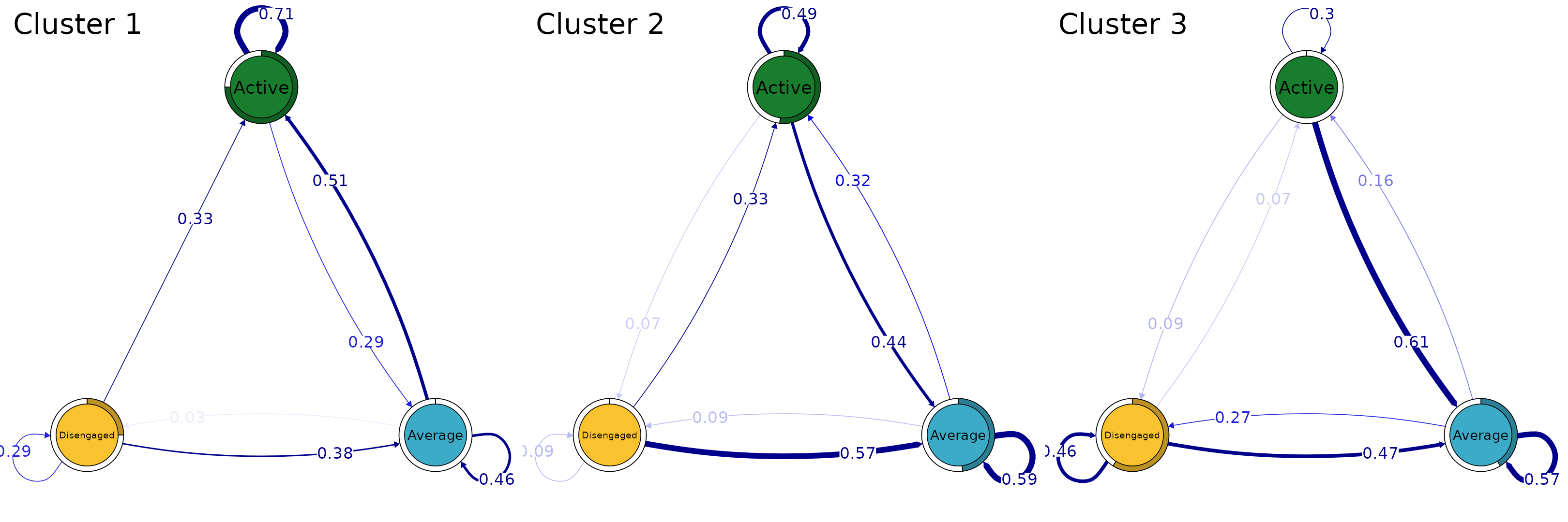
We can also plot the cluster-specific transitions

layout(t(1:3))
plot(tna_model_clus, vsize = 20, edge.label.cex = 2)

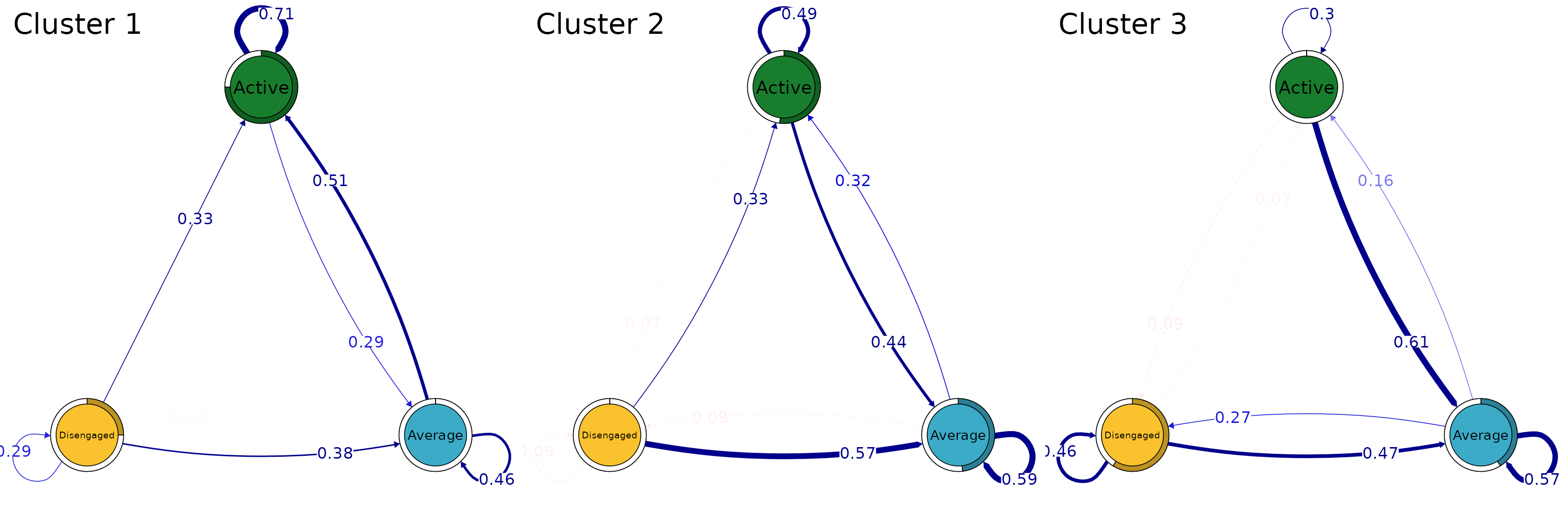
Just like ordinary TNA models, we can prune the rare transitions

pruned_clus <- prune(tna_model_clus, threshold = 0.1)

and plot the cluster transitions after pruning

layout(t(1:3))
plot(pruned_clus, vsize = 20, edge.label.cex = 2)

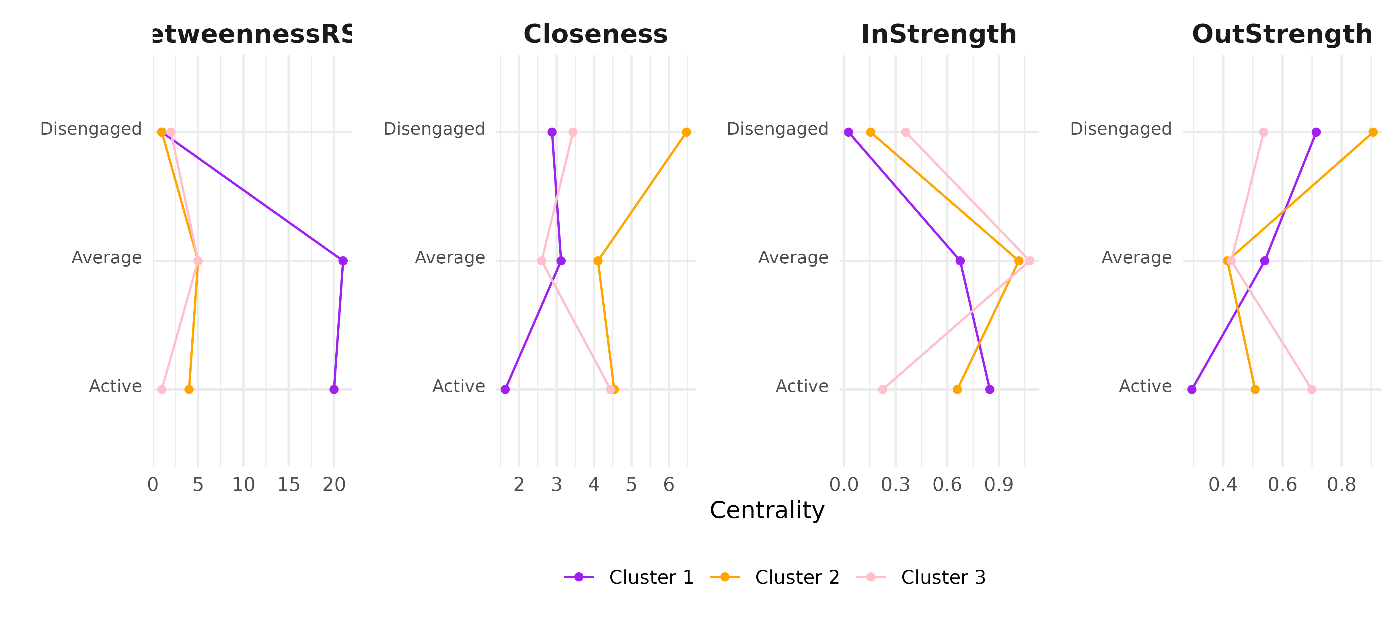
Centrality measures can also be computed for each cluster directly.

centrality_measures <- c(
  "BetweennessRSP",
  "Closeness",
  "InStrength",
  "OutStrength"
)
centralities_per_cluster <- centralities(
  tna_model_clus,
  measures = centrality_measures
)
plot(
  centralities_per_cluster, ncol = 4,
  colors = c("purple", "orange", "pink")
)