# Install 'tna' package from CRAN if needed (uncomment if required).
# install.packages("tna")

# Load packages
library("tna")

# Load example data provided within the 'tna' package,
# representing group regulatory interactions
data(group_regulation)

# Run FTNA on 'group_regulation' data using raw counts of
# transitions ("absolute" type) and print the result
model <- ftna(group_regulation)

# Print the output to inspect the model
print(model)
#> State Labels :
#>
#>    adapt, cohesion, consensus, coregulate, discuss, emotion, monitor, plan, synthesis
#>
#> Transition Frequency Matrix :
#>
#>            adapt cohesion consensus coregulate discuss emotion monitor plan
#> adapt          0      139       243         11      30      61      17    8
#> cohesion       5       46       844        202     101     196      56  239
#> consensus     30       94       519       1188    1190     460     295 2505
#>            synthesis
#> adapt              0
#> cohesion           6
#> consensus         48
#>  [ reached 'max' / getOption("max.print") -- omitted 6 rows ]
#>
#> Initial Probabilities :
#>
#>      adapt   cohesion  consensus coregulate    discuss    emotion    monitor
#>      0.011      0.060      0.214      0.019      0.175      0.151      0.144
#>       plan  synthesis
#>      0.204      0.019
# Calculate the Transition Network Analysis (TNA) on the group_regulation
# data with scaled weights between 0 and 1
model_scaled <- ftna(group_regulation, scaling = "minmax")
print(model_scaled) # Print the FTNA model with scaled weights
#> State Labels :
#>
#>    adapt, cohesion, consensus, coregulate, discuss, emotion, monitor, plan, synthesis
#>
#> Transition Frequency Matrix :
#>
#>             adapt cohesion consensus coregulate discuss emotion monitor   plan
#> adapt      0.0000   0.0555     0.097     0.0044   0.012   0.024  0.0068 0.0032
#> cohesion   0.0020   0.0184     0.337     0.0806   0.040   0.078  0.0224 0.0954
#> consensus  0.0120   0.0375     0.207     0.4743   0.475   0.184  0.1178 1.0000
#>            synthesis
#> adapt         0.0000
#> cohesion      0.0024
#> consensus     0.0192
#>  [ reached 'max' / getOption("max.print") -- omitted 6 rows ]
#>
#> Initial Probabilities :
#>
#>      adapt   cohesion  consensus coregulate    discuss    emotion    monitor
#>      0.011      0.060      0.214      0.019      0.175      0.151      0.144
#>       plan  synthesis
#>      0.204      0.019
Plotting
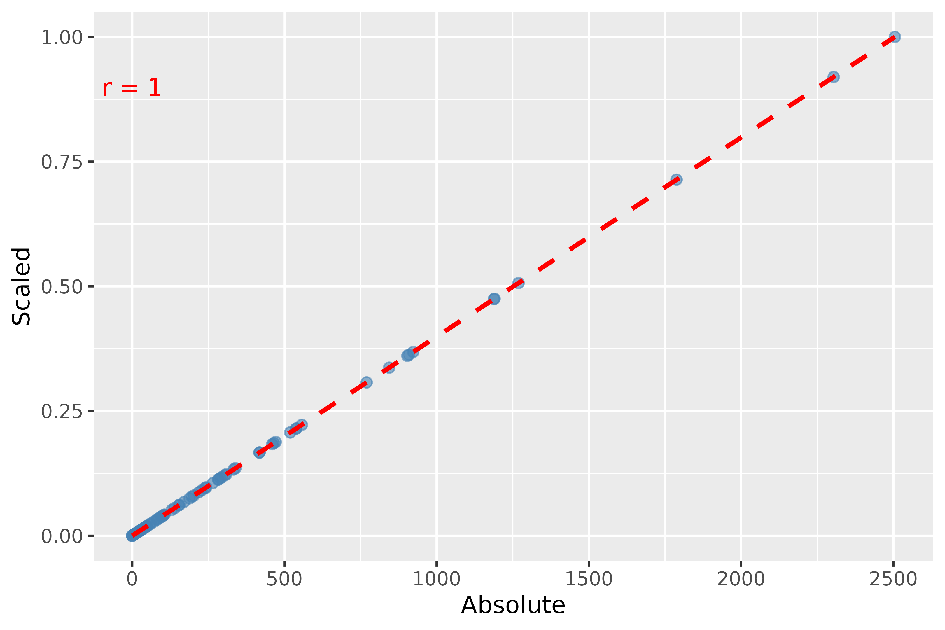
# Plotting the two weights together to see if the scaling distorts the data

# Combine weights from absolute and scaled models into a data frame for plotting
weights_data <- data.frame(
  Absolute = as.vector(model$weights), # Extract absolute weights as a vector
  Scaled = as.vector(model_scaled$weights) # Extract scaled weights as a vector
)
corr <- cor(weights_data$Absolute, weights_data$Scaled, method = c("pearson")) |>
  round(digits = 2)

# Create a scatter plot comparing absolute vs. scaled weights
plot_abs_scaled <- ggplot(weights_data, aes(x = Absolute, y = Scaled)) +
  geom_point(color = "steelblue", alpha = 0.6, size = 2) +  # Add points with specified aesthetics
  geom_smooth(formula = y ~ x, method = "lm", color = "red", linetype = "dashed") + # Add a linear trend line
  # geom_smooth(method = lm, formula = y ~ x, se = FALSE) +
  geom_text(x = 0.1, y = 0.9, label = paste0('r = ', corr), color = 'red')
  # stat_cor(aes(label = after_stat(r.label)), label.x = 0.1, label.y = 0.9,
  #          size = 4, color = "black", method = "spearman") + # Display Spearman correlation
  labs(x = "Absolute Weights", y = "Scaled Weights") + # Label axes
  theme_minimal() # Apply a minimal theme for the plot
#> NULL

# Display the scatter plot
plot_abs_scaled
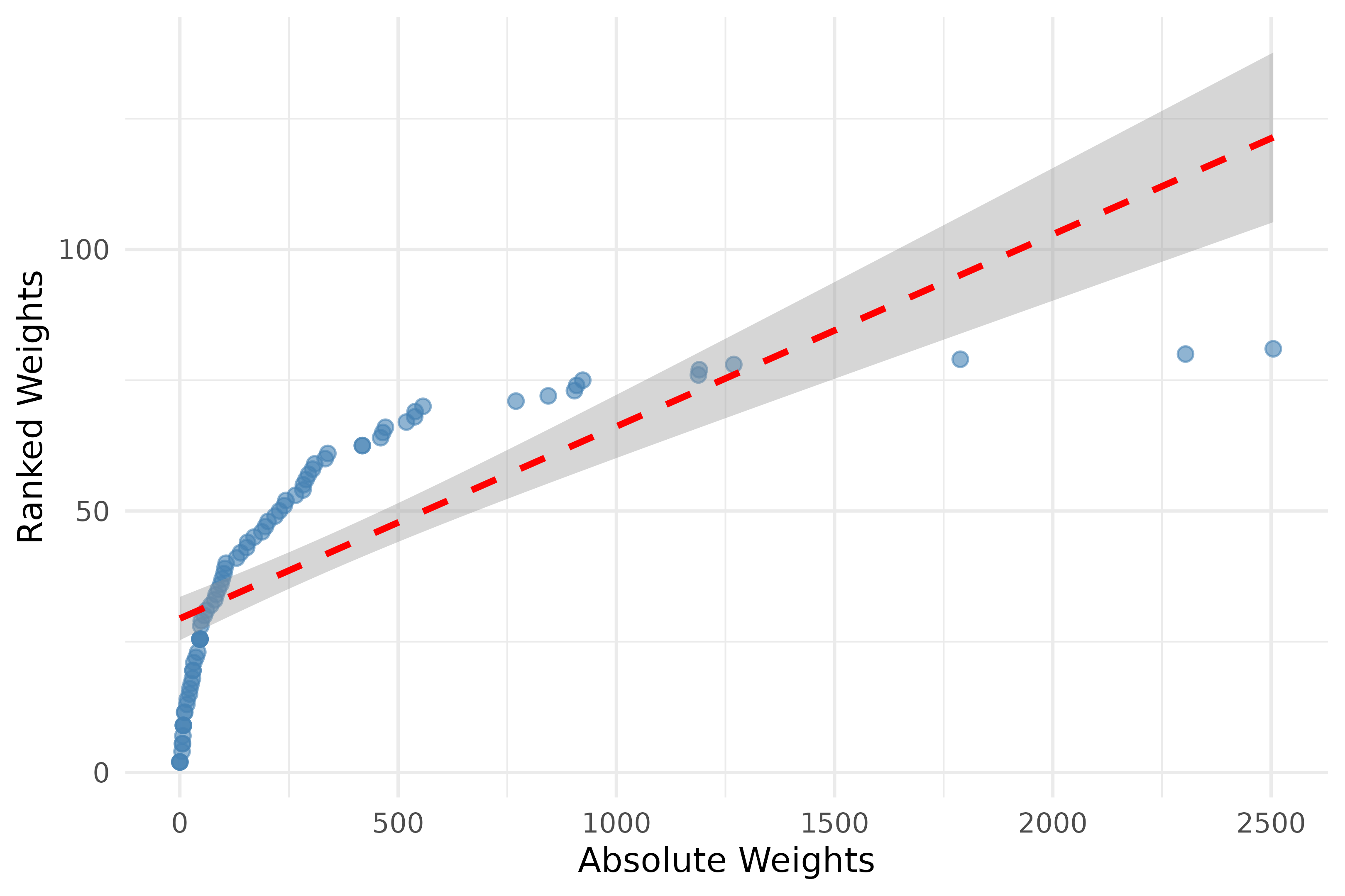
# Calculate the Transition Network Analysis (TNA) on the `group_regulation`
# data with ranked weights
model_ranked <- ftna(group_regulation, scaling = "rank")
print(model_ranked) # Print the FTNA model with ranked weights
# Combine weights from absolute and ranked models into a data frame for plotting
weights_data <- data.frame(
  Absolute = as.vector(model$weights), # Extract absolute weights as a vector
  Ranked = as.vector(model_ranked$weights) # Extract ranked weights as a vector
)

# Create a scatter plot comparing Absolute vs. Ranked weights with correlation annotations
plot_abs_ranked <- ggplot(weights_data, aes(x = Absolute, y = Ranked)) +
  geom_point(color = "steelblue", alpha = 0.6, size = 2) +  # Add points with specified aesthetics
  geom_smooth(formula = y ~ x, method = "lm", color = "red", linetype = "dashed") +  # Add a linear trend line
  # stat_cor(aes(label = paste("Spearman: ", round(after_stat(r), 2))),
  #          method = "spearman", label.x = 0.1, label.y = 0.9, size = 4, color = "black") + # Spearman correlation annotation
  # stat_cor(aes(label = paste("Pearson: ", round(after_stat(r), 2))),
  #          method = "pearson", label.x = 0.1, label.y = 0.8, size = 4, color = "darkgreen") + # Pearson correlation annotation
  labs(x = "Absolute Weights", y = "Ranked Weights") + # Label axes
  theme_minimal() # Apply a minimal theme for the plot

# Display the scatter plot
plot_abs_ranked
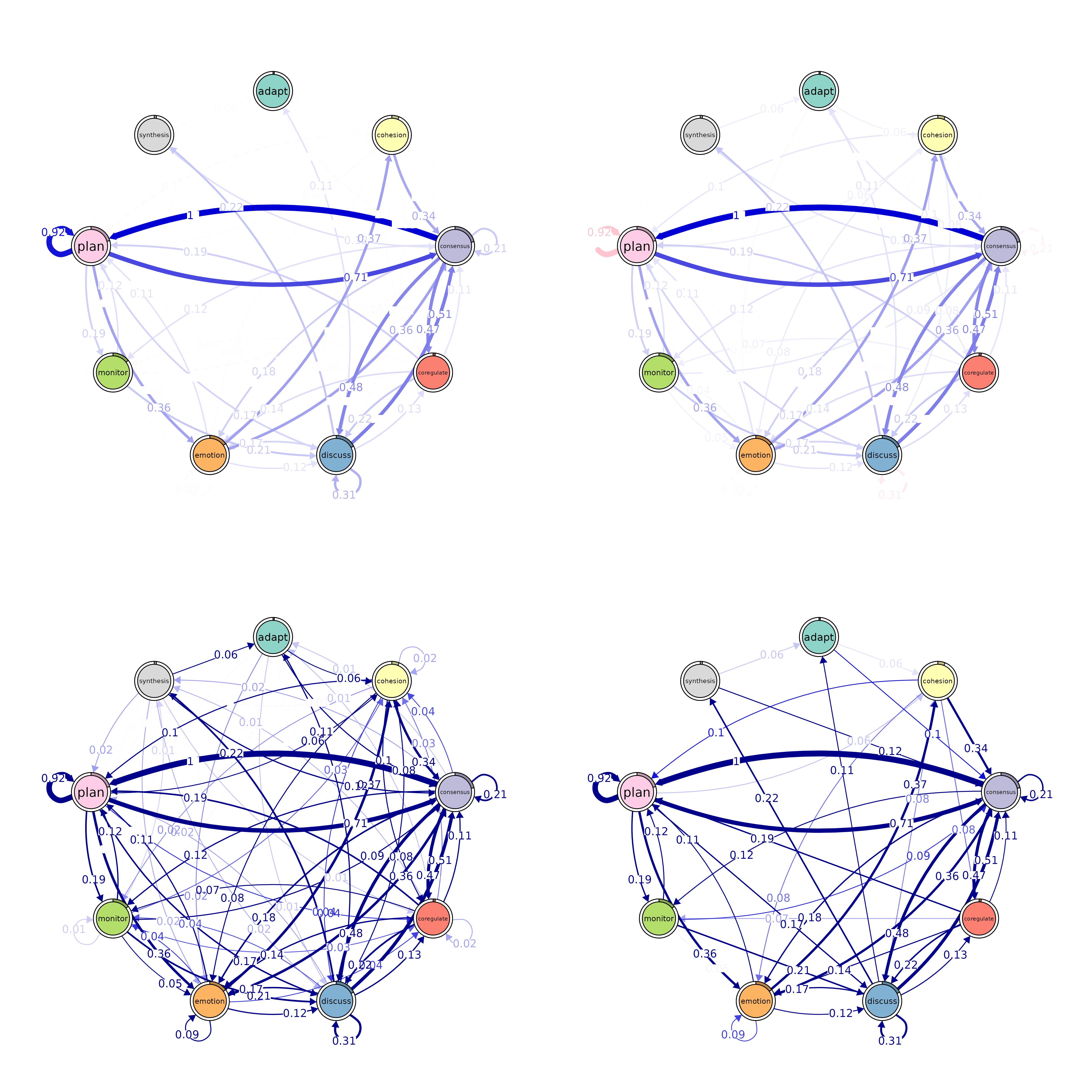
Pruning
layout(matrix(1:4, ncol = 2))
# Pruning with different methods
pruned_threshold <- prune(model_scaled, method = "threshold", threshold = 0.1)
pruned_lowest <- prune(model_scaled, method = "lowest", lowest = 0.15)
pruned_disparity <- prune(model_scaled, method = "disparity", alpha = 0.5)
# Plotting for comparison
plot(pruned_threshold)
#> Registered S3 method overwritten by 'cograph':
#> method from
#> plot.tna_bootstrap tna
plot(pruned_lowest)
plot(pruned_disparity)
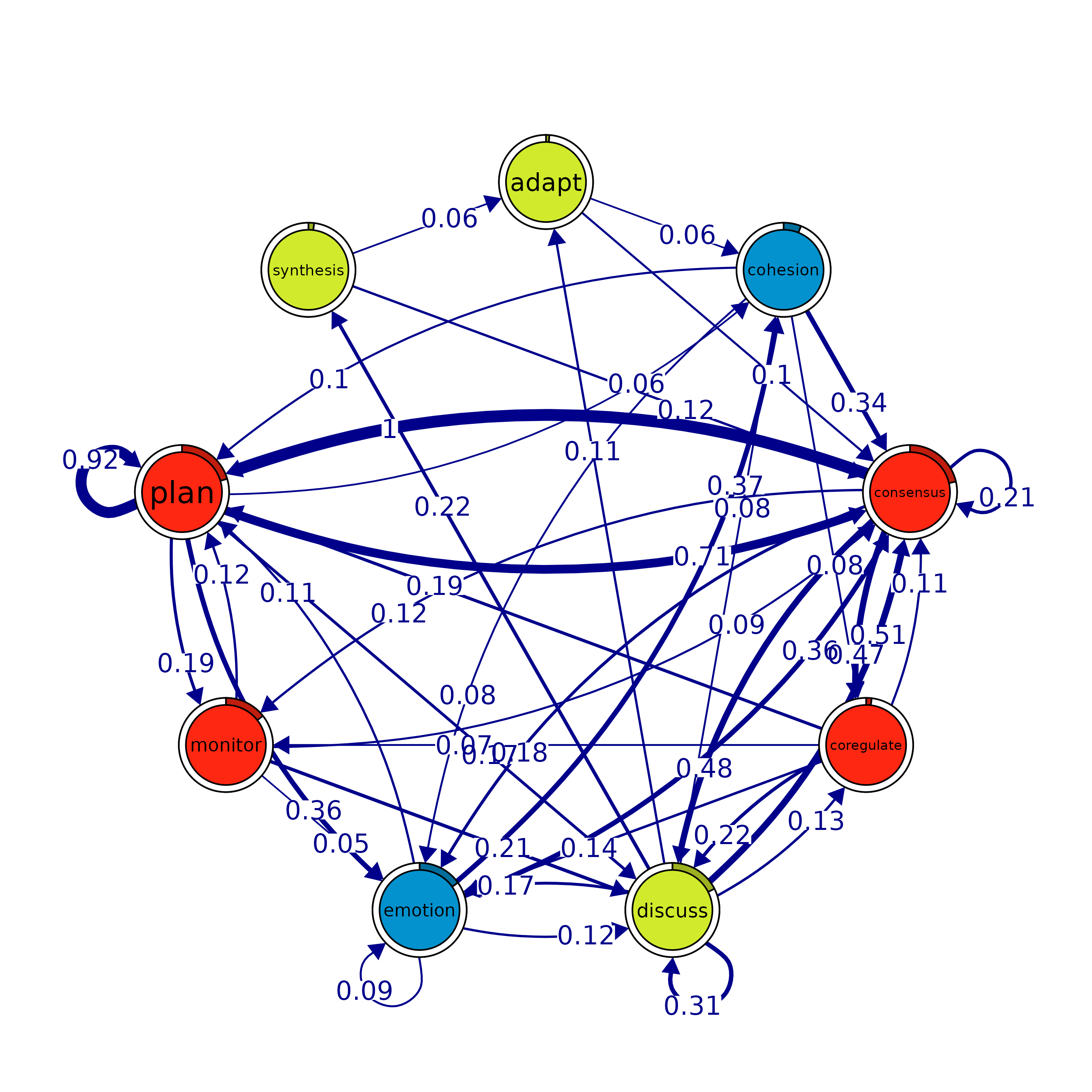
plot(model_scaled)
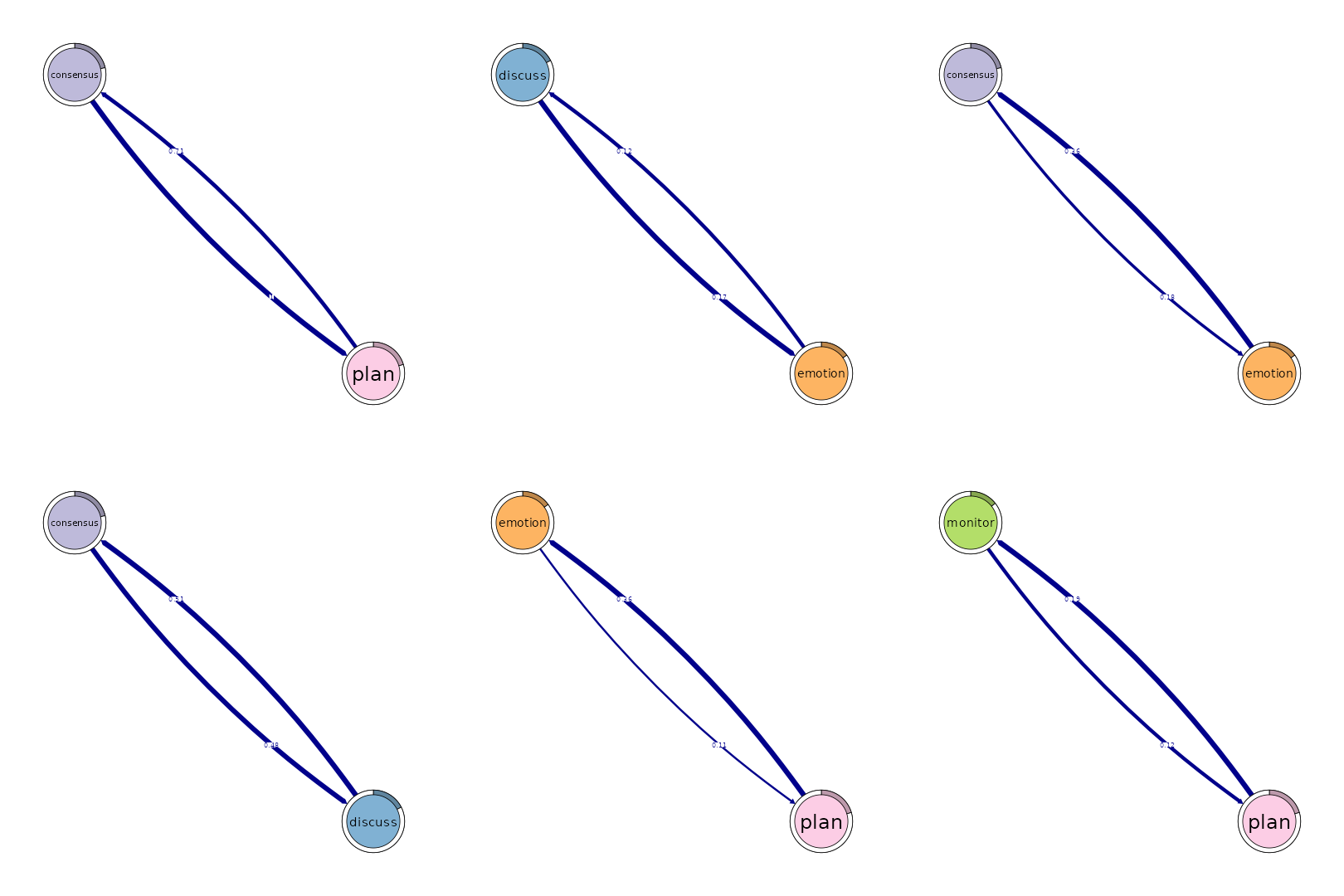
Patterns
# Identify 2-cliques (dyads) from the FTNA model with a weight threshold,
# excluding loops in visualization.
# A 2-clique represents a pair of nodes that are strongly connected based on
# the specified weight threshold.
layout(matrix(1:6, ncol = 3))
cliques_of_two <- cliques(
  model_scaled,      # The FTNA model with scaled edge weights
  size = 2,          # Looking for pairs of connected nodes (dyads)
  threshold = 0.1    # Only include edges with weights greater than 0.1
)

# Print and visualize the identified 2-cliques (dyads)
print(cliques_of_two)  # Display details of 2-cliques
#> Number of 2-cliques = 8 (weight threshold = 0.1)
#> Showing 6 cliques starting from clique number 1
#>
#> Clique 1
#>           consensus plan
#> consensus      0.21 1.00
#> plan           0.71 0.92
#>
#> Clique 2
#>           consensus discuss
#> consensus      0.21    0.48
#> discuss        0.51    0.31
#>
#> Clique 3
#>         discuss emotion
#> discuss    0.31   0.167
#> emotion    0.12   0.087
#>
#> Clique 4
#>         emotion plan
#> emotion   0.087 0.11
#> plan      0.361 0.92
#>
#> Clique 5
#>           consensus emotion
#> consensus      0.21   0.184
#> emotion        0.36   0.087
#>
#> Clique 6
#>         monitor plan
#> monitor    0.01 0.12
#> plan       0.19 0.92
plot(cliques_of_two, ask = F)   # Visualize 2-cliques in the network
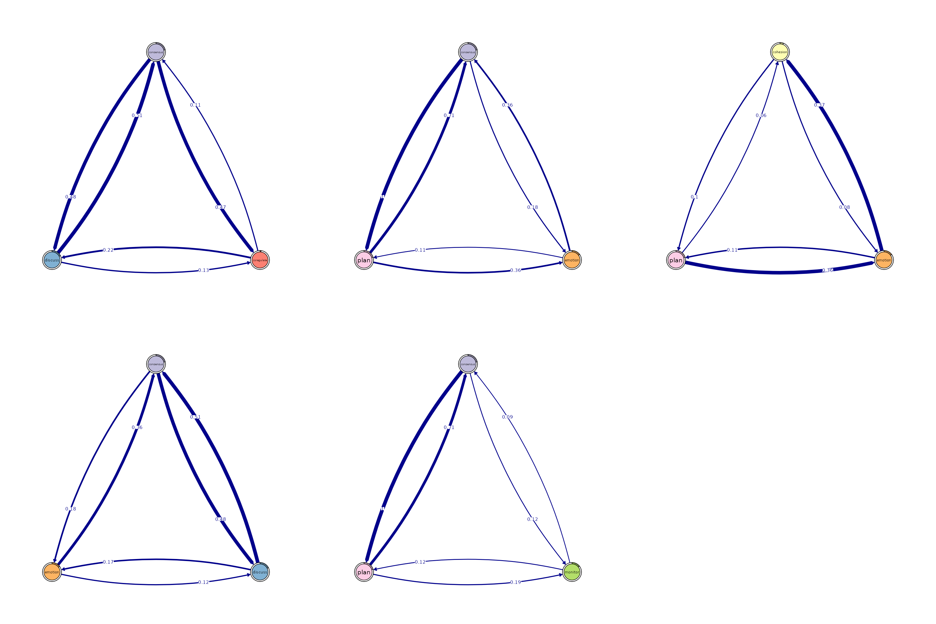
layout(matrix(1:6, ncol = 3))
# Identify 3-cliques (triads) from the FTNA model.
# A 3-clique is a fully connected set of three nodes, indicating a strong
# triplet structure.
cliques_of_three <- cliques(
  model_scaled,      # The FTNA model with scaled edge weights
  size = 3,          # Looking for triplets of fully connected nodes (triads)
  threshold = 0.05   # Only include edges with weights greater than 0.05
)

# Print and visualize the identified 3-cliques (triads)
# Uncomment the code below to view the results
print(cliques_of_three) # Display details of 3-cliques
#> Number of 3-cliques = 5 (weight threshold = 0.05)
#> Showing 5 cliques starting from clique number 1
#>
#> Clique 1
#>            consensus coregulate discuss
#> consensus       0.21      0.474    0.48
#> coregulate      0.11      0.018    0.22
#> discuss         0.51      0.133    0.31
#>
#> Clique 2
#>           consensus discuss emotion
#> consensus      0.21    0.48   0.184
#> discuss        0.51    0.31   0.167
#> emotion        0.36    0.12   0.087
#>
#> Clique 3
#>           consensus emotion plan
#> consensus      0.21   0.184 1.00
#> emotion        0.36   0.087 0.11
#> plan           0.71   0.361 0.92
#>
#> Clique 4
#>           consensus monitor plan
#> consensus     0.207    0.12 1.00
#> monitor       0.091    0.01 0.12
#> plan          0.714    0.19 0.92
#>
#> Clique 5
#>          cohesion emotion  plan
#> cohesion    0.018   0.078 0.095
#> emotion     0.368   0.087 0.113
#> plan        0.062   0.361 0.920
plot(cliques_of_three, ask = FALSE)  # Visualize 3-cliques in the network
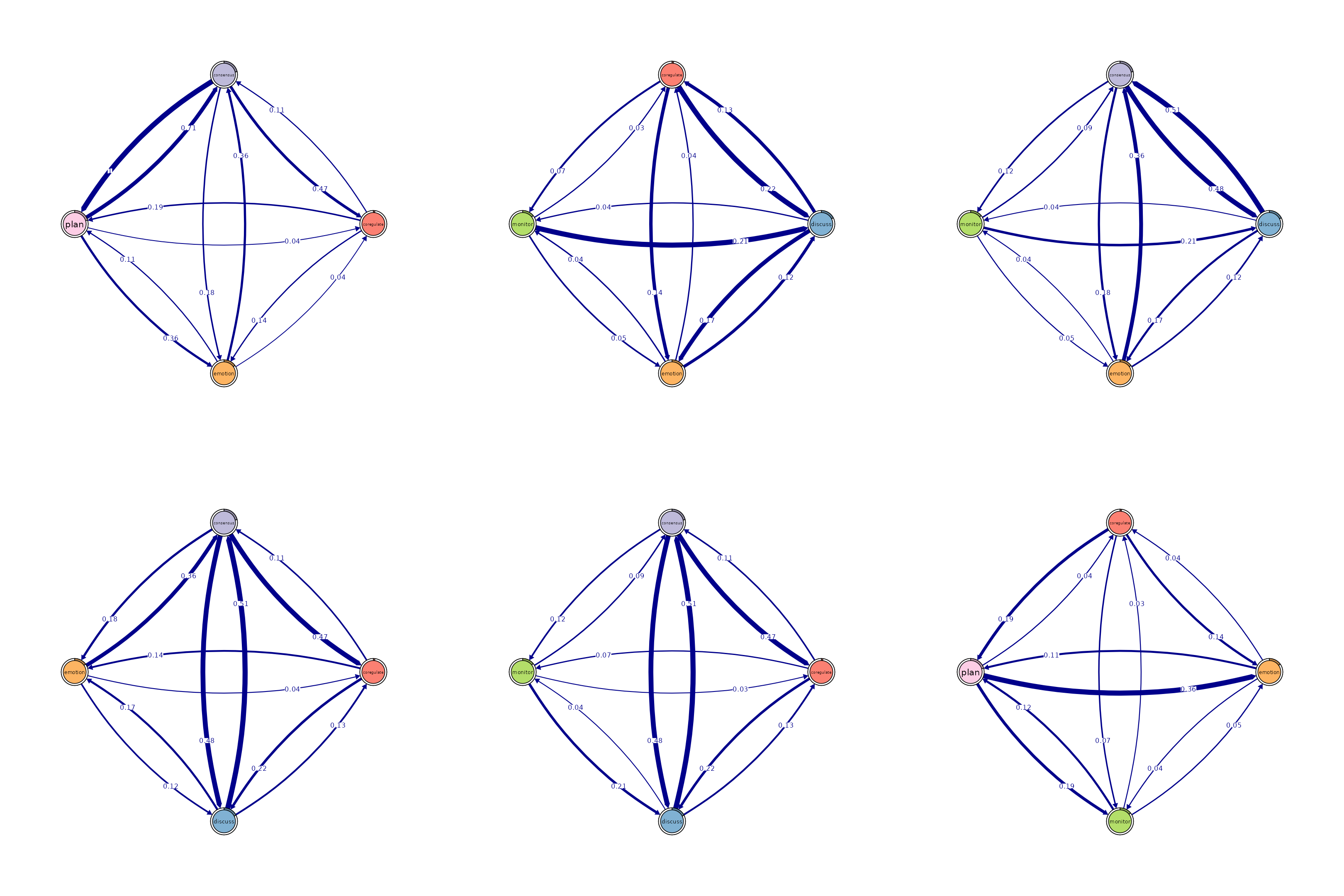
layout(matrix(1:6, ncol = 3))
# Identify 4-cliques (quadruples) from the FTNA model.
# A 4-clique includes four nodes where each node is connected to every other
# node in the group.
# Uncomment the code below to view the results
cliques_of_four <- cliques(
  model_scaled,      # The FTNA model with scaled edge weights
  size = 4,          # Looking for quadruples of fully connected nodes (4-cliques)
  threshold = 0.03   # Only include edges with weights greater than 0.03
)

# Print and visualize the identified 4-cliques (quadruples)
# Uncomment the code below to view the results
print(cliques_of_four)  # Display details of 4-cliques
#> Number of 4-cliques = 11 (weight threshold = 0.03)
#> Showing 6 cliques starting from clique number 1
#>
#> Clique 1
#>            consensus coregulate emotion plan
#> consensus       0.21      0.474   0.184 1.00
#> coregulate      0.11      0.018   0.135 0.19
#> emotion         0.36      0.039   0.087 0.11
#> plan            0.71      0.042   0.361 0.92
#>
#> Clique 2
#>            consensus coregulate discuss emotion
#> consensus       0.21      0.474    0.48   0.184
#> coregulate      0.11      0.018    0.22   0.135
#> discuss         0.51      0.133    0.31   0.167
#> emotion         0.36      0.039    0.12   0.087
#>
#> Clique 3
#>            coregulate discuss emotion monitor
#> coregulate      0.018    0.22   0.135   0.068
#> discuss         0.133    0.31   0.167   0.035
#> emotion         0.039    0.12   0.087   0.041
#> monitor         0.033    0.21   0.052   0.010
#>
#> Clique 4
#>            consensus coregulate discuss monitor
#> consensus      0.207      0.474    0.48   0.118
#> coregulate     0.106      0.018    0.22   0.068
#> discuss        0.507      0.133    0.31   0.035
#> monitor        0.091      0.033    0.21   0.010
#>
#> Clique 5
#>           consensus discuss emotion monitor
#> consensus     0.207    0.48   0.184   0.118
#> discuss       0.507    0.31   0.167   0.035
#> emotion       0.363    0.12   0.087   0.041
#> monitor       0.091    0.21   0.052   0.010
#>
#> Clique 6
#>            coregulate emotion monitor plan
#> coregulate      0.018   0.135   0.068 0.19
#> emotion         0.039   0.087   0.041 0.11
#> monitor         0.033   0.052   0.010 0.12
#> plan            0.042   0.361   0.186 0.92
plot(cliques_of_four, ask = FALSE)   # Visualize 4-cliques in the network
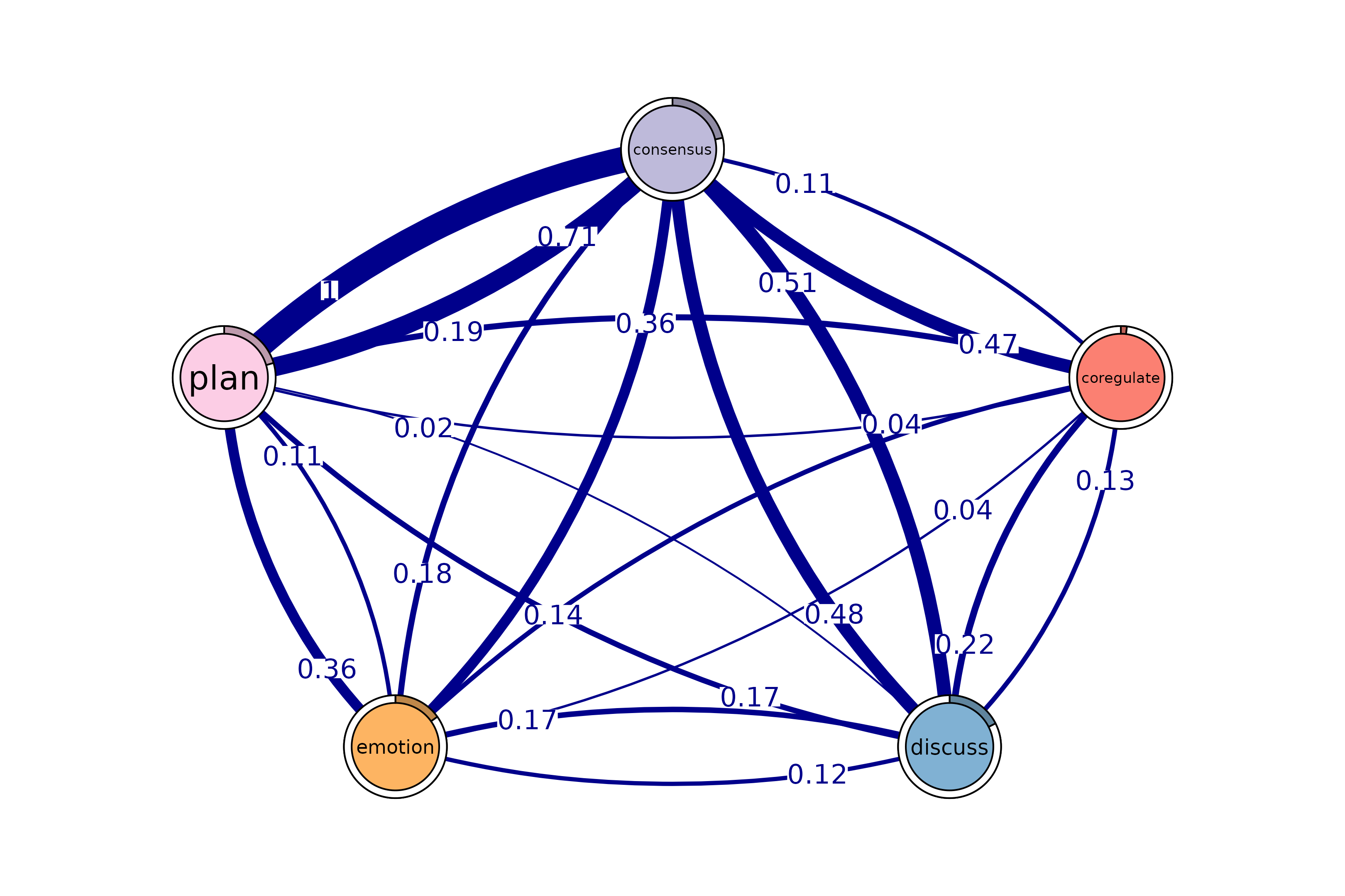
# Identify 5-cliques (quintuples) from the FTNA model, summing edge weights.
# Here, the sum of edge weights in both directions must meet the specified
# threshold for inclusion.
# Uncomment the code below to view the results
cliques_of_five <- cliques(
  model_scaled,      # The FTNA model with scaled edge weights
  size = 5,          # Looking for quintuples of fully connected nodes (5-cliques)
  threshold = 0.1,   # Only edges with total bidirectional weights greater than 0.1
  sum_weights = TRUE # Sum edge weight in both directions when computing  threshold
)

# Print and visualize the identified 5-cliques (quintuples)
print(cliques_of_five)  # Display details of 5-cliques
#> Number of 5-cliques = 1 (weight threshold = 0.1)
#> Showing 1 cliques starting from clique number 1
#>
#> Clique 1
#>            consensus coregulate discuss emotion  plan
#> consensus       0.21      0.474    0.48   0.184 1.000
#> coregulate      0.11      0.018    0.22   0.135 0.188
#> discuss         0.51      0.133    0.31   0.167 0.018
#> emotion         0.36      0.039    0.12   0.087 0.113
#> plan            0.71      0.042    0.17   0.361 0.920
plot(cliques_of_five, ask = FALSE)   # Visualize 5-cliques in the network
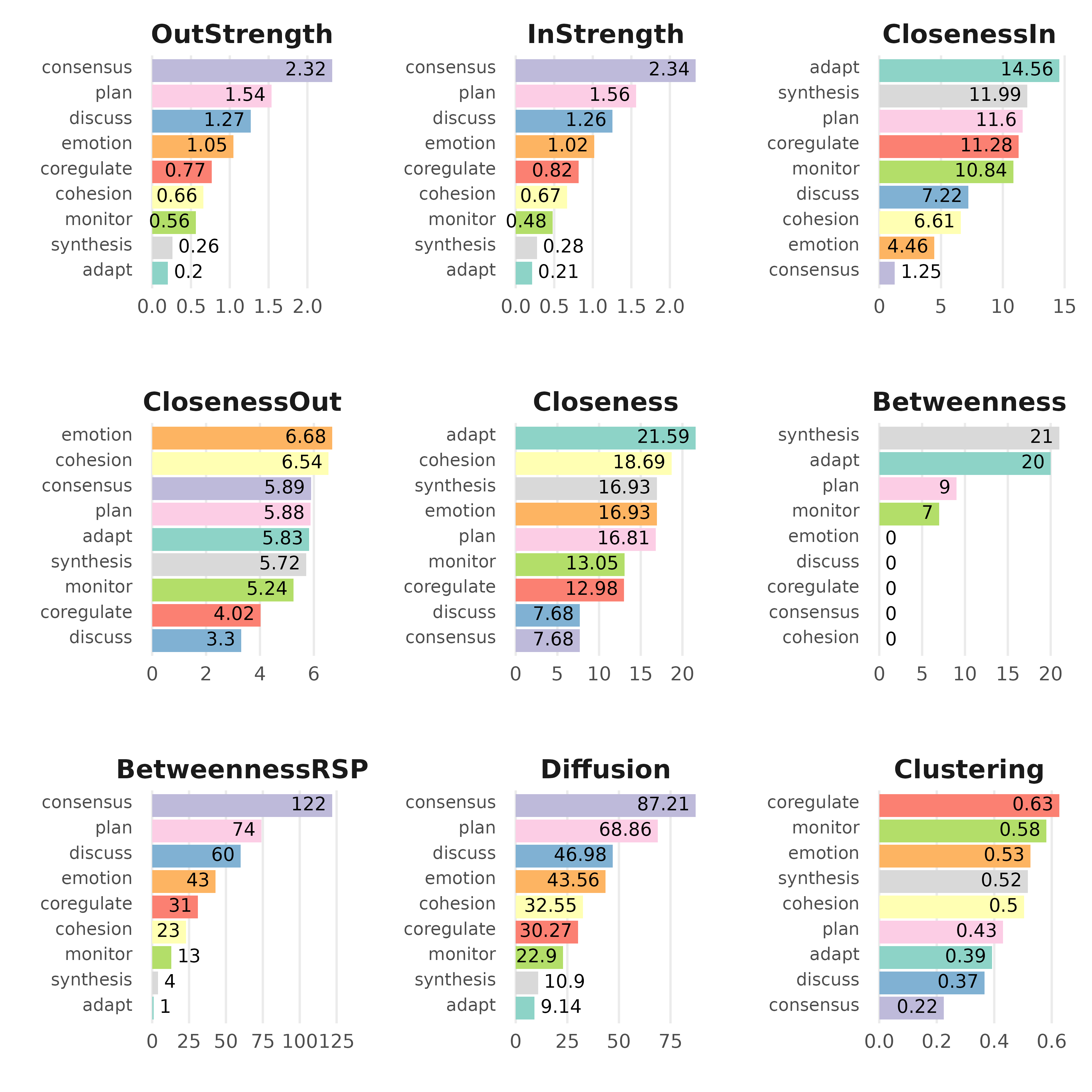
Node level measures
# Compute centrality measures for the FTNA model
centrality_measures <- centralities(model_scaled)

# Print the calculated centrality measures in the FTNA model
print(centrality_measures)
#> # A tibble: 9 × 10
#>   state      OutStrength InStrength ClosenessIn ClosenessOut Closeness Betweenness
#> * <fct>            <dbl>      <dbl>       <dbl>        <dbl>     <dbl>       <dbl>
#> 1 adapt            0.203      0.212     0.00967      0.00901    0.0104           0
#> 2 cohesion         0.658      0.667     0.0128       0.0176     0.0193           0
#> 3 consensus        2.32       2.34      0.0245       0.0254     0.0294          39
#> 4 coregulate       0.768      0.818     0.0196       0.0148     0.0205           0
#> 5 discuss          1.27       1.26      0.0210       0.0222     0.0272          19
#> 6 emotion          1.05       1.02      0.0159       0.0195     0.0207           7
#> 7 monitor          0.562      0.480     0.0124       0.0135     0.0154           0
#> 8 plan             1.54       1.56      0.0221       0.0236     0.0263          18
#> 9 synthesis        0.260      0.275     0.0137       0.0104     0.0147           0
#> # ℹ 3 more variables: BetweennessRSP <dbl>, Diffusion <dbl>, Clustering <dbl>
plot(centrality_measures)
# Convert the FTNA model to an igraph object and
# calculate HITS (Hub and Authority) scores
hits_results <- igraph::hits_scores(as.igraph(model_scaled))

# Extract the hub and authority scores from the HITS results for further analysis
hub_scores <- hits_results$hub
authority_scores <- hits_results$authority
# Print the hub and authority scores to view influential nodes
print(hub_scores)
#>      adapt   cohesion  consensus coregulate    discuss    emotion    monitor
#>      0.056      0.240      0.955      0.256      0.377      0.305      0.189
#>       plan  synthesis
#>      1.000      0.074
print(authority_scores)
#>      adapt   cohesion  consensus coregulate    discuss    emotion    monitor
#>      0.033      0.129      0.672      0.293      0.437      0.344      0.174
#>       plan  synthesis
#>      1.000      0.056
Comparing Models
# Create FTNA for the high-achievers subset (rows 1 to 1000)
Hi <- ftna(group_regulation[1:1000, ], scaling = "minmax")
# Create FTNA for the low-achievers subset (rows 1001 to 2000)
Lo <- ftna(group_regulation[1001:2000, ], scaling = "minmax")
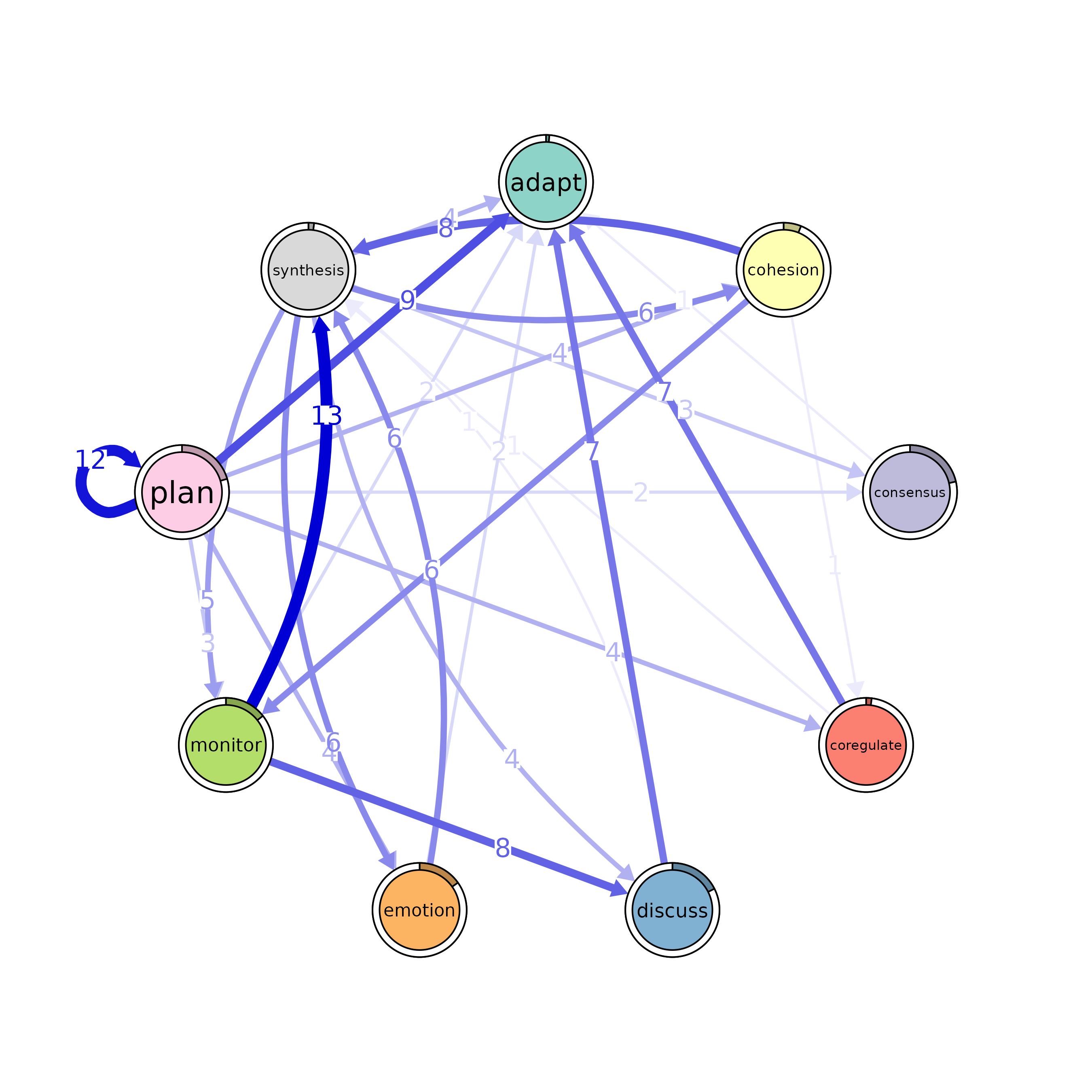
# Plot a comparison of the "Hi" and "Lo" models
# The 'minimum' parameter is set to 0.001, so edges with weights >= 0.001 are shown
plot_compare(Hi, Lo, minimum = 0.0001)
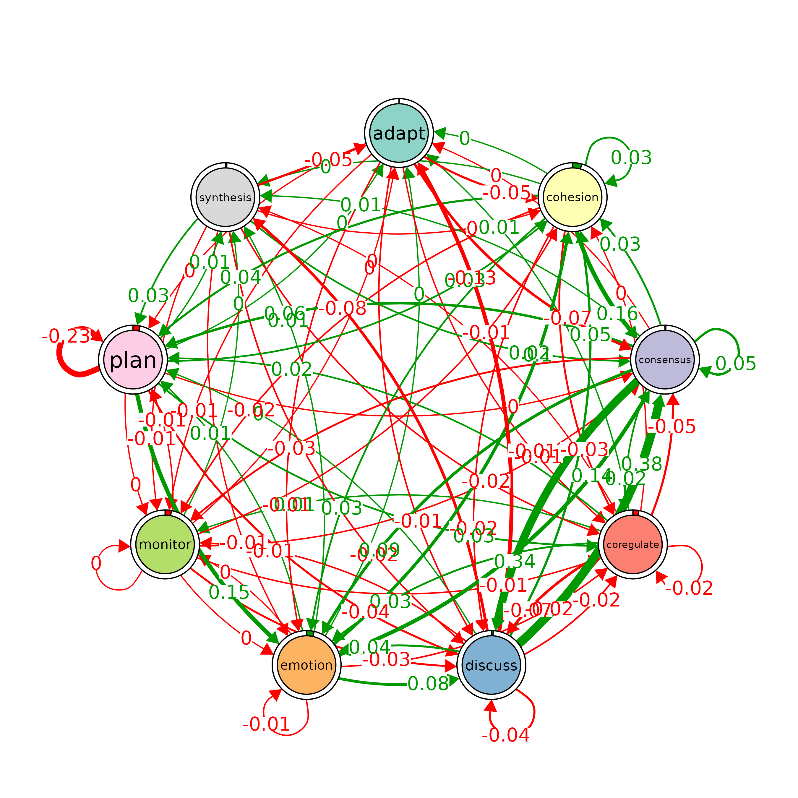
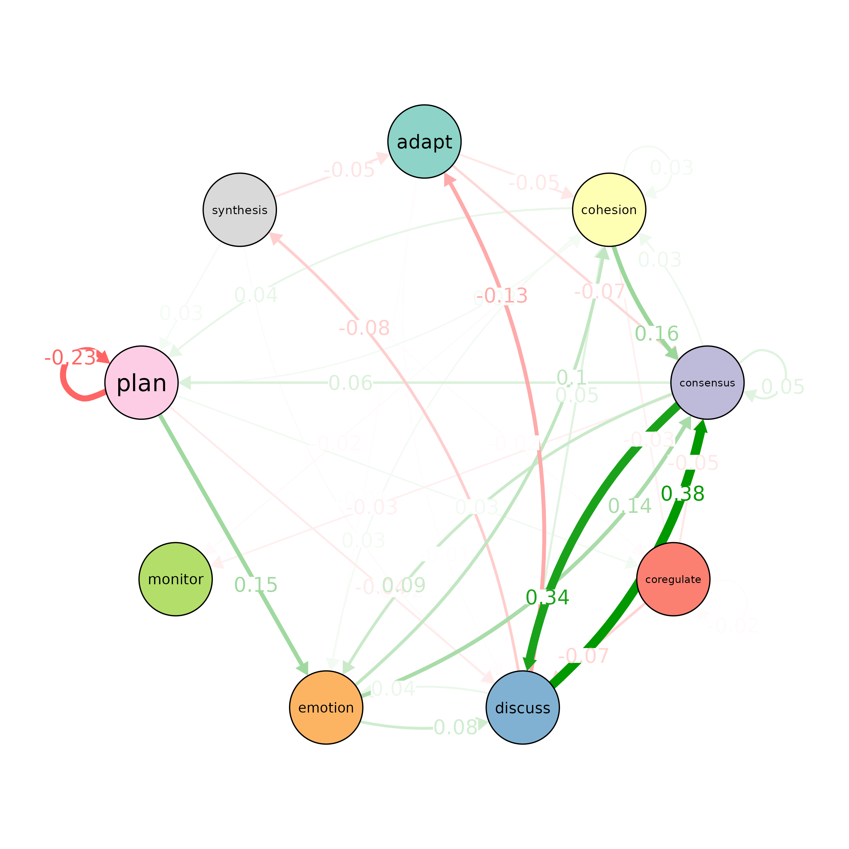
# Run a permutation test to determine statistical significance of
# differences between "Hi" and "Lo"
# The 'it' parameter is set to 1000, meaning 1000 permutations are performed
Permutation <- permutation_test(Hi, Lo, it = 1000)

# Plot the significant differences identified in the permutation test
plot(Permutation)