Tutorial of TNA with R
This is a short tutorial of the tna package. We begin by
loading the package and the example data set
group_regulation.
Building tna Model
TNA models can be built with the tna function, which
accepts several types of data such a sequence data, data frames or
matrices.
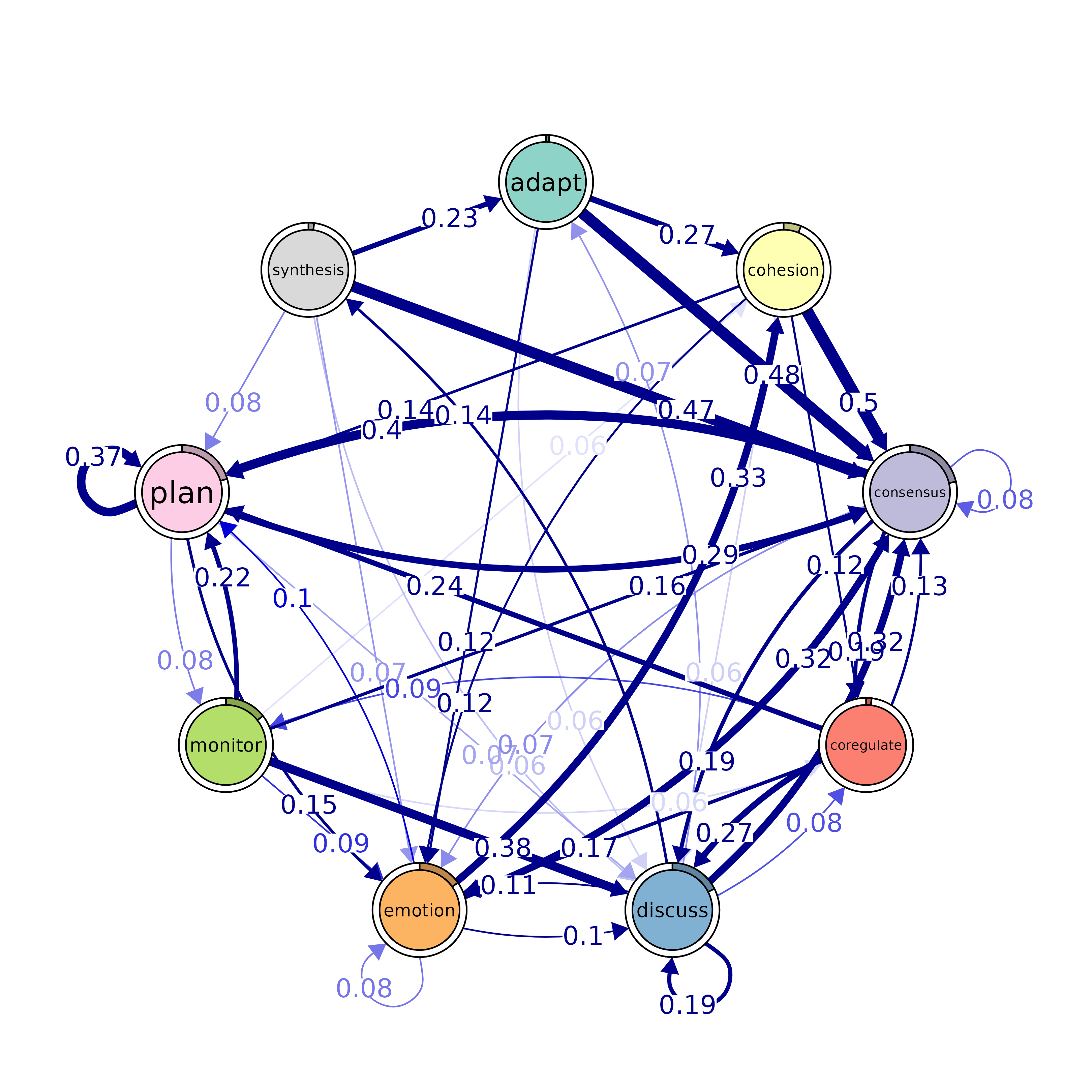
Plotting and interpreting tna models
Pruning and retaining edges that “matter”
layout(matrix(1:4, ncol = 2, byrow = TRUE))
# Pruning with different methods (using comparable parameters)
pruned_threshold <- prune(model, method = "threshold", threshold = 0.15)
pruned_lowest <- prune(model, method = "lowest", lowest = 0.15)
pruned_disparity <- prune(model, method = "disparity", level = 0.5)

# Plotting for comparison
plot(pruned_threshold)
plot(pruned_lowest)
plot(pruned_disparity)
plot(model)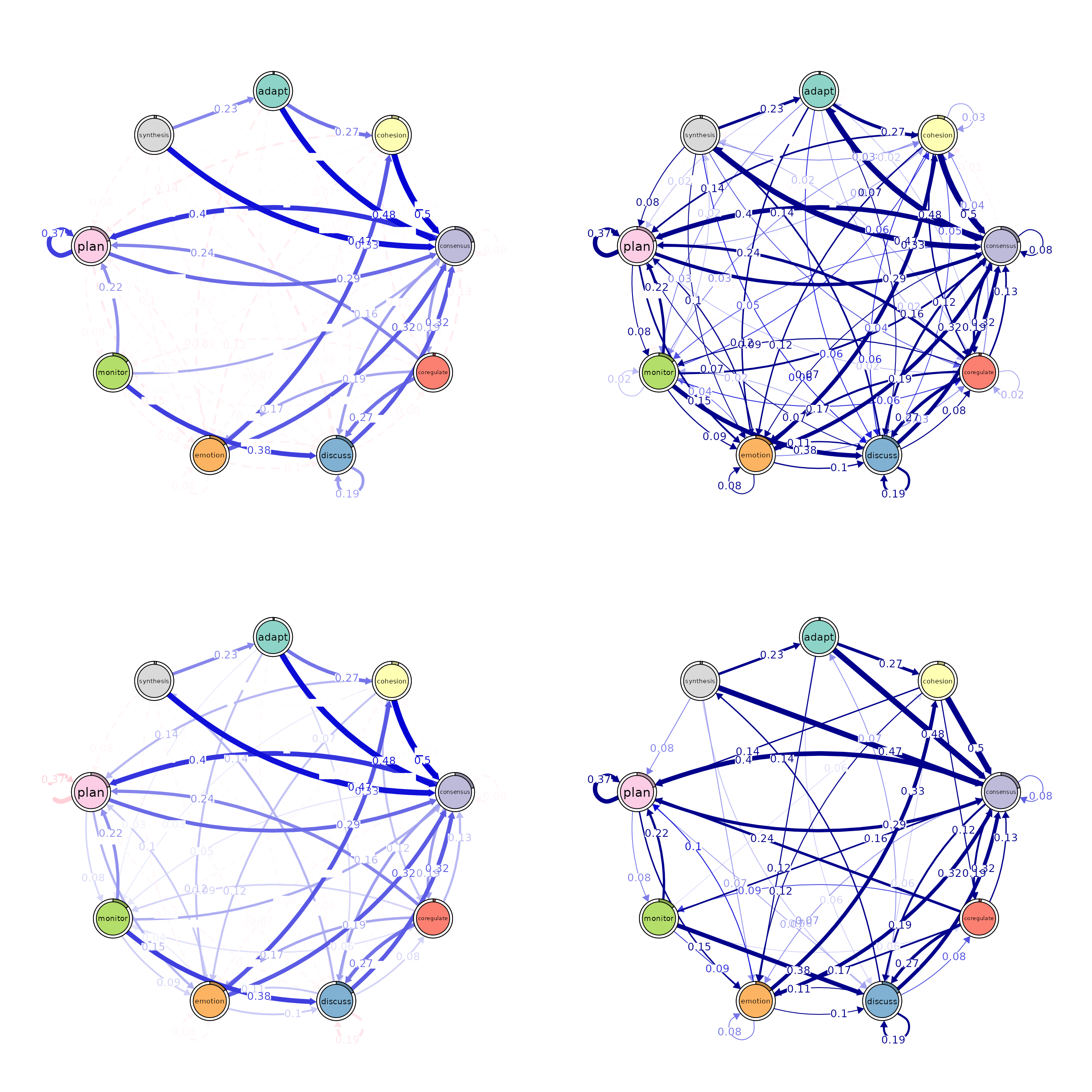
Patterns
layout(t(1:2))
# Identify 2-cliques (dyads) from the TNA model, excluding loops in the visualization
# A clique of size 2 is essentially a pair of connected nodes
cliques_of_two <- cliques(
  model,
  size = 2,
  threshold = 0.15  # Only consider edges with weight > 0.15
)
print(cliques_of_two)
#> Number of 2-cliques = 2 (weight threshold = 0.15)
#> Showing 2 cliques starting from clique number 1
#>
#> Clique 1
#>           consensus plan
#> consensus     0.082 0.40
#> plan          0.290 0.37
#>
#> Clique 2
#>           consensus discuss
#> consensus     0.082    0.19
#> discuss       0.321    0.19
plot(cliques_of_two, ask = FALSE)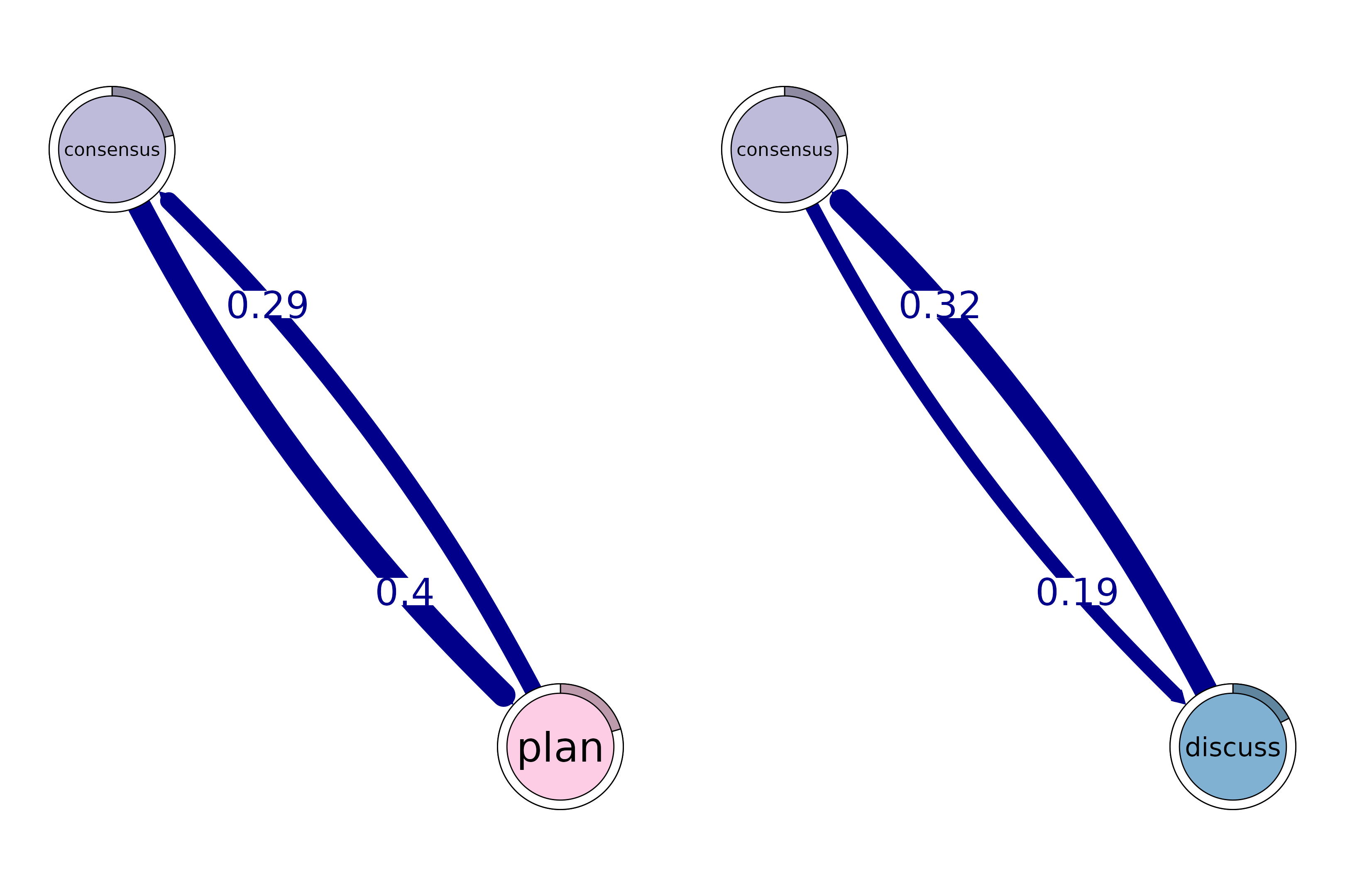
layout(t(1:3))
# Identify 3-cliques (triads) from the TNA_Model
# A clique of size 3 means a fully connected triplet of nodes
cliques_of_three <- cliques(
  model,
  size = 3,
  threshold = 0.05 # Only consider edges with weight > 0.05
)
print(cliques_of_three)
#> Number of 3-cliques = 3 (weight threshold = 0.05)
#> Showing 3 cliques starting from clique number 1
#>
#> Clique 1
#>           consensus discuss emotion
#> consensus     0.082    0.19   0.073
#> discuss       0.321    0.19   0.106
#> emotion       0.320    0.10   0.077
#>
#> Clique 2
#>           consensus emotion plan
#> consensus     0.082   0.073 0.40
#> emotion       0.320   0.077 0.10
#> plan          0.290   0.147 0.37
#>
#> Clique 3
#>            consensus coregulate discuss
#> consensus      0.082      0.188    0.19
#> coregulate     0.135      0.023    0.27
#> discuss        0.321      0.084    0.19
plot(cliques_of_three, ask = FALSE)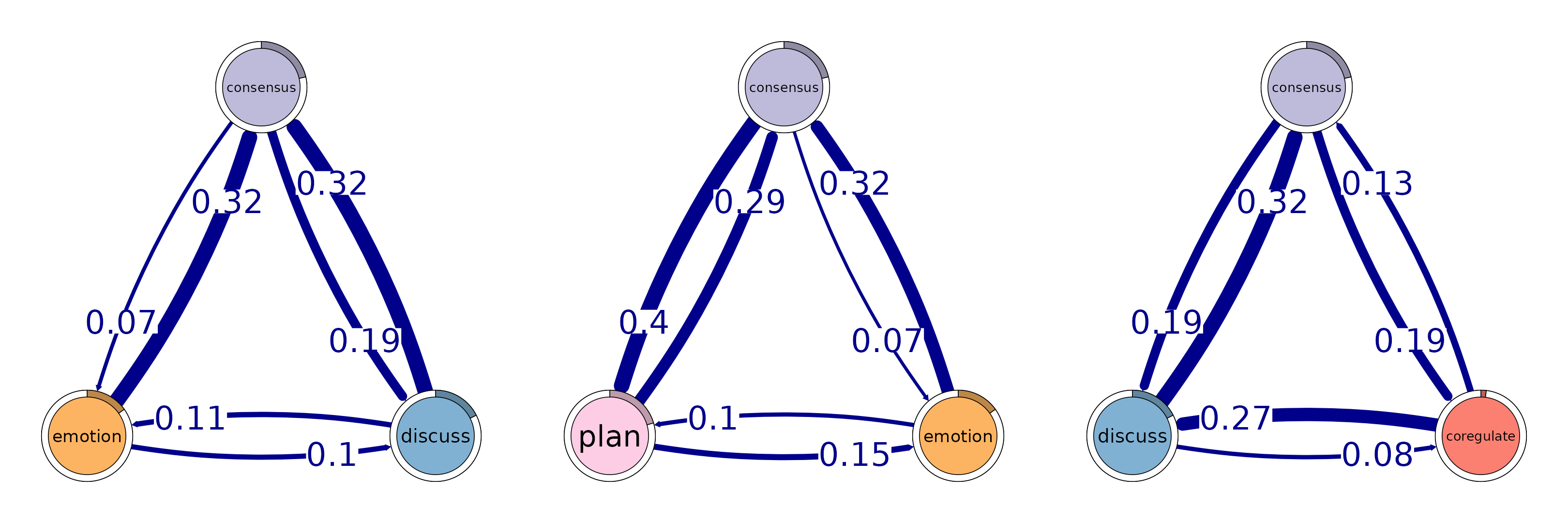
# Identify 4-cliques (quadruples) from the TNA_Model
# A clique of size 4 means four nodes that are all mutually connected
cliques_of_four <- cliques(
  model,
  size = 4,
  threshold = 0.035 # Only consider edges with weight > 0.03
)
print(cliques_of_four)
#> Number of 4-cliques = 1 (weight threshold = 0.035)
#> Showing 1 cliques starting from clique number 1
#>
#> Clique 1
#>           consensus emotion monitor plan
#> consensus     0.082   0.073   0.047 0.40
#> emotion       0.320   0.077   0.036 0.10
#> monitor       0.159   0.091   0.018 0.22
#> plan          0.290   0.147   0.076 0.37
plot(cliques_of_four, ask = FALSE)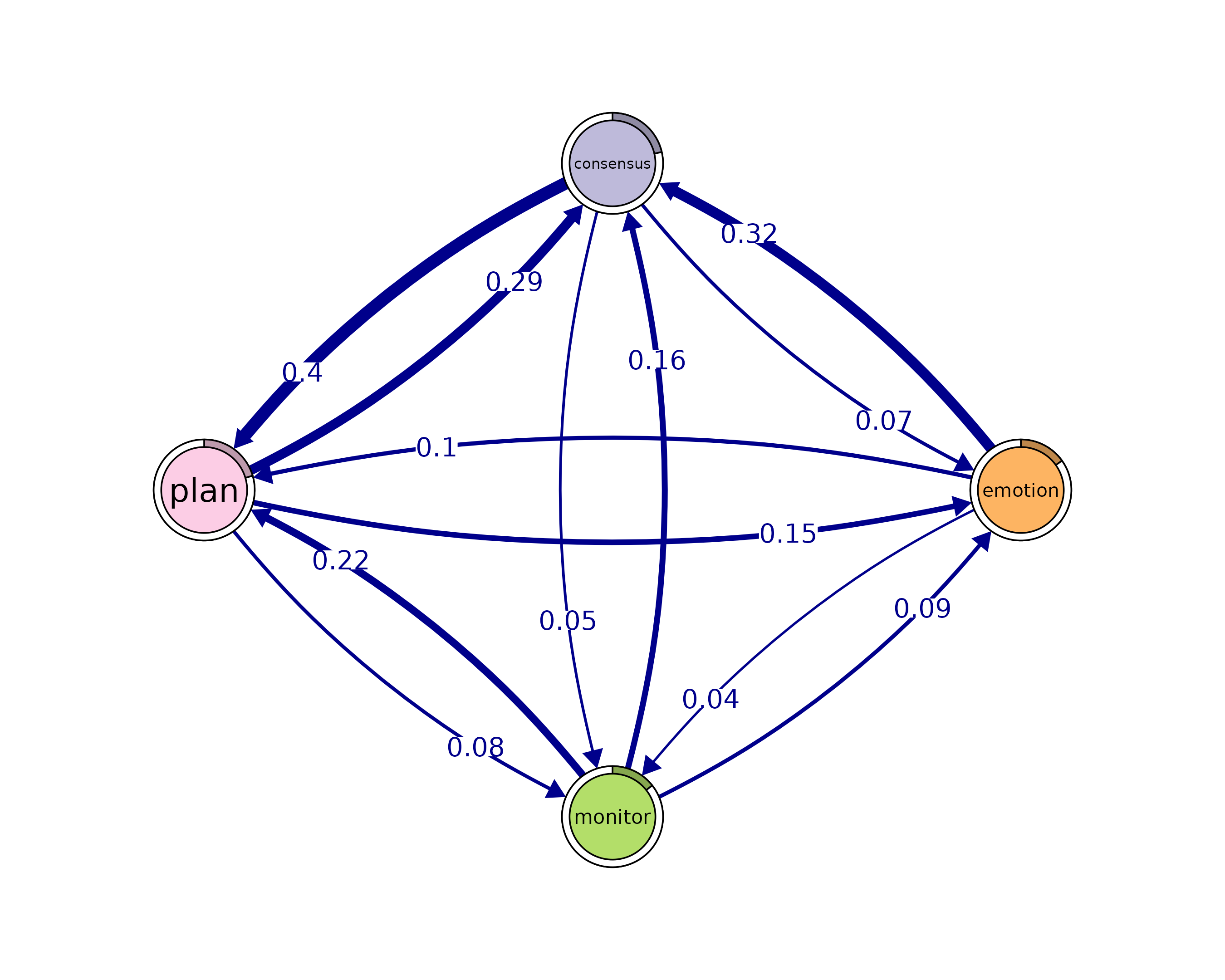
Centralities
Node-level measures
# Compute centrality measures for the TNA model
Centralities <- centralities(model)

# Visualize the centrality measures
plot(Centralities)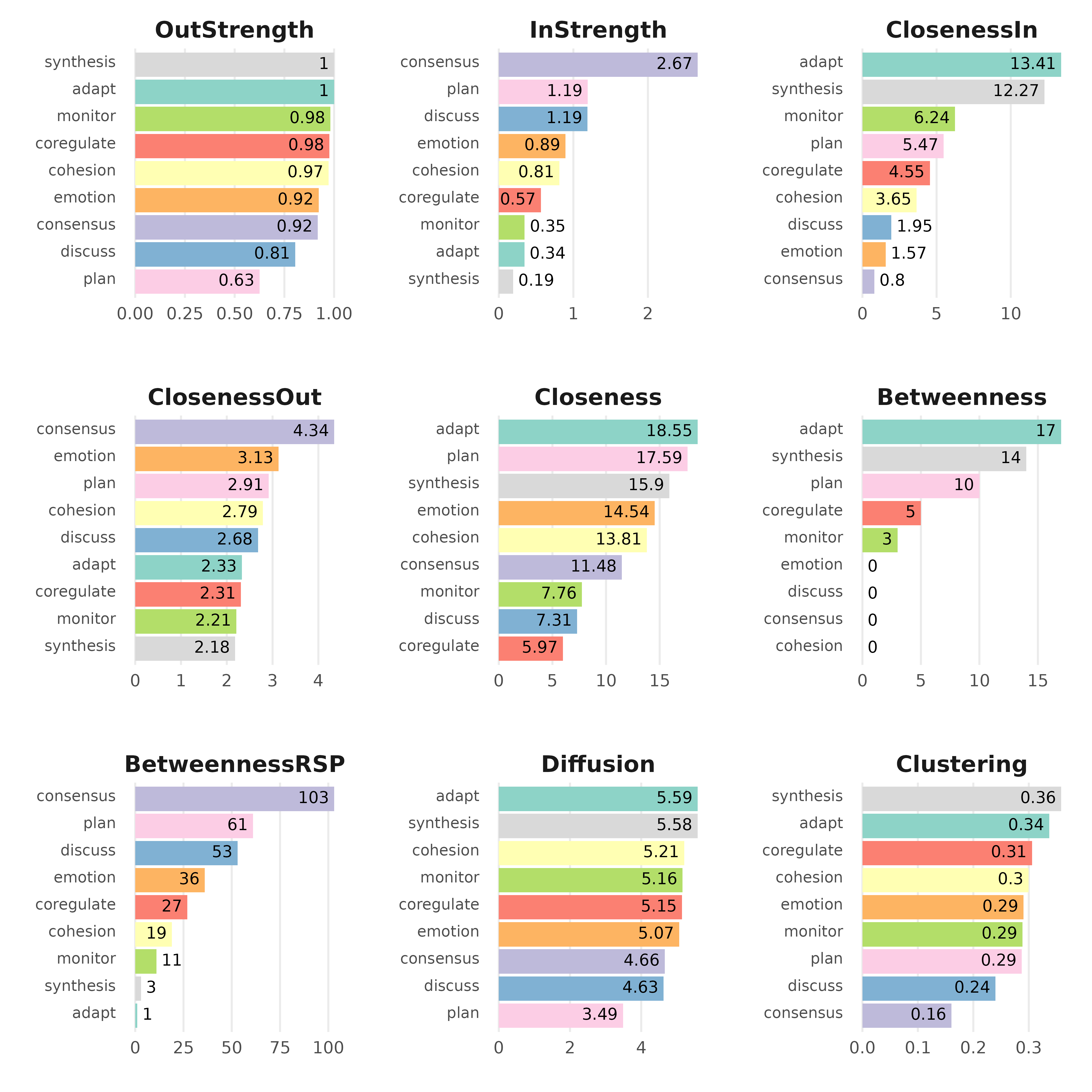
# Calculate hub scores and the authority scores for the network
hits_scores <- igraph::hits_scores(as.igraph(model))
hub_scores <- hits_scores$hub
authority_scores <- hits_scores$authority

# Print the calculated hub and authority scores for further analysis
print(hub_scores)
#>      adapt   cohesion  consensus coregulate    discuss    emotion    monitor
#>       0.96       1.00       0.65       0.69       0.74       0.82       0.74
#>       plan  synthesis
#>       0.87       0.90
print(authority_scores)
#>      adapt   cohesion  consensus coregulate    discuss    emotion    monitor
#>      0.122      0.301      1.000      0.195      0.439      0.333      0.122
#>       plan  synthesis
#>      0.511      0.059
Edge-level measures
# Edge betweenness
Edge_betweeness <- betweenness_network(model)
plot(Edge_betweeness)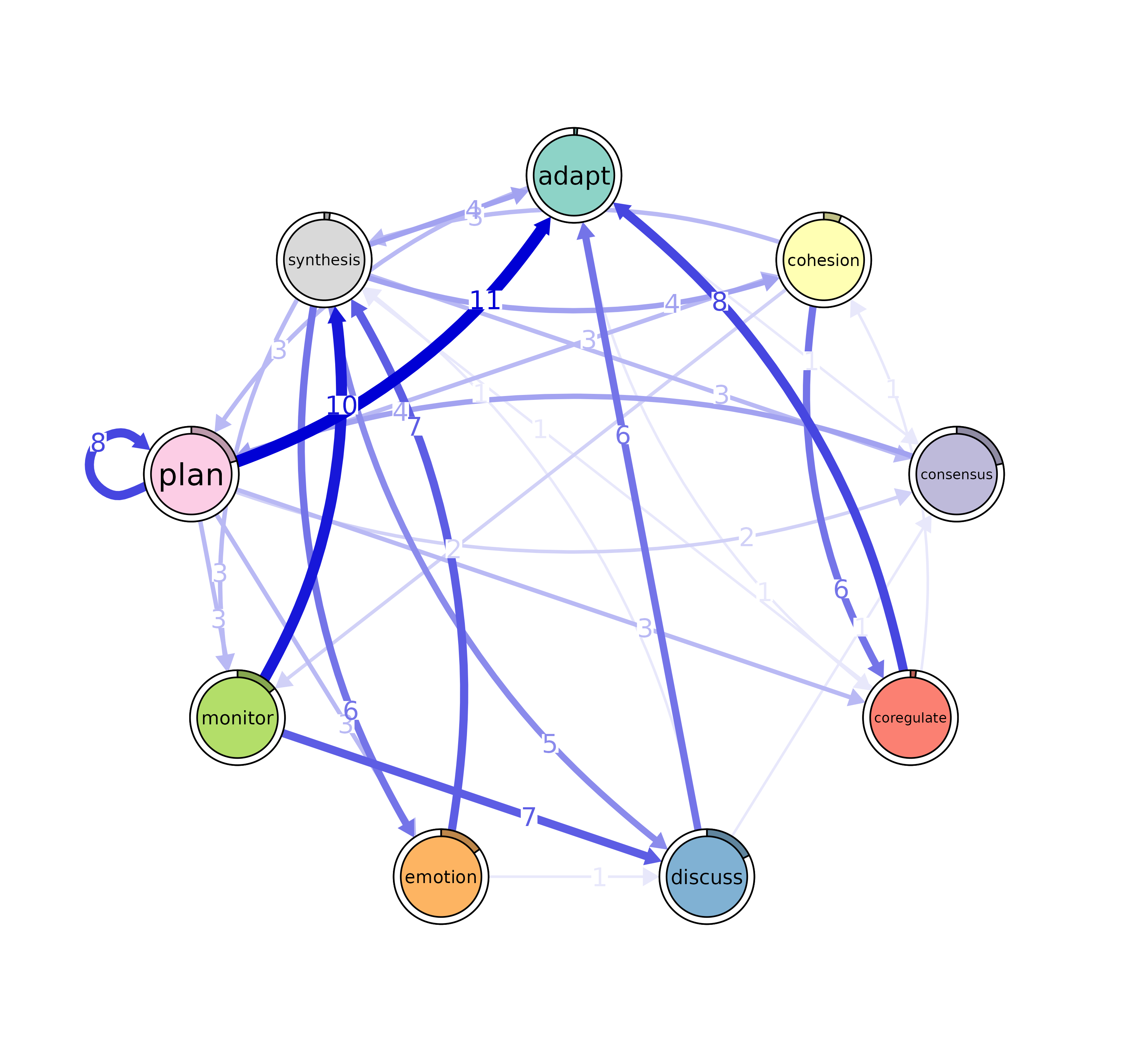
Community finding
communities <- communities(model)
print(communities)
#> Number of communities found by each algorithm
#>
#>         walktrap      fast_greedy       label_prop          infomap
#>                1                3                1                1
#> edge_betweenness    leading_eigen        spinglass
#>                1                3                2
#>
#> Community assignments
#>
#>       state walktrap fast_greedy label_prop infomap edge_betweenness leading_eigen
#> 1     adapt        1           1          1       1                1             1
#> 2  cohesion        1           1          1       1                1             1
#> 3 consensus        1           1          1       1                1             2
#>   spinglass
#> 1         1
#> 2         1
#> 3         1
#>  [ reached 'max' / getOption("max.print") -- omitted 6 rows ]
plot(communities, method = "leading_eigen")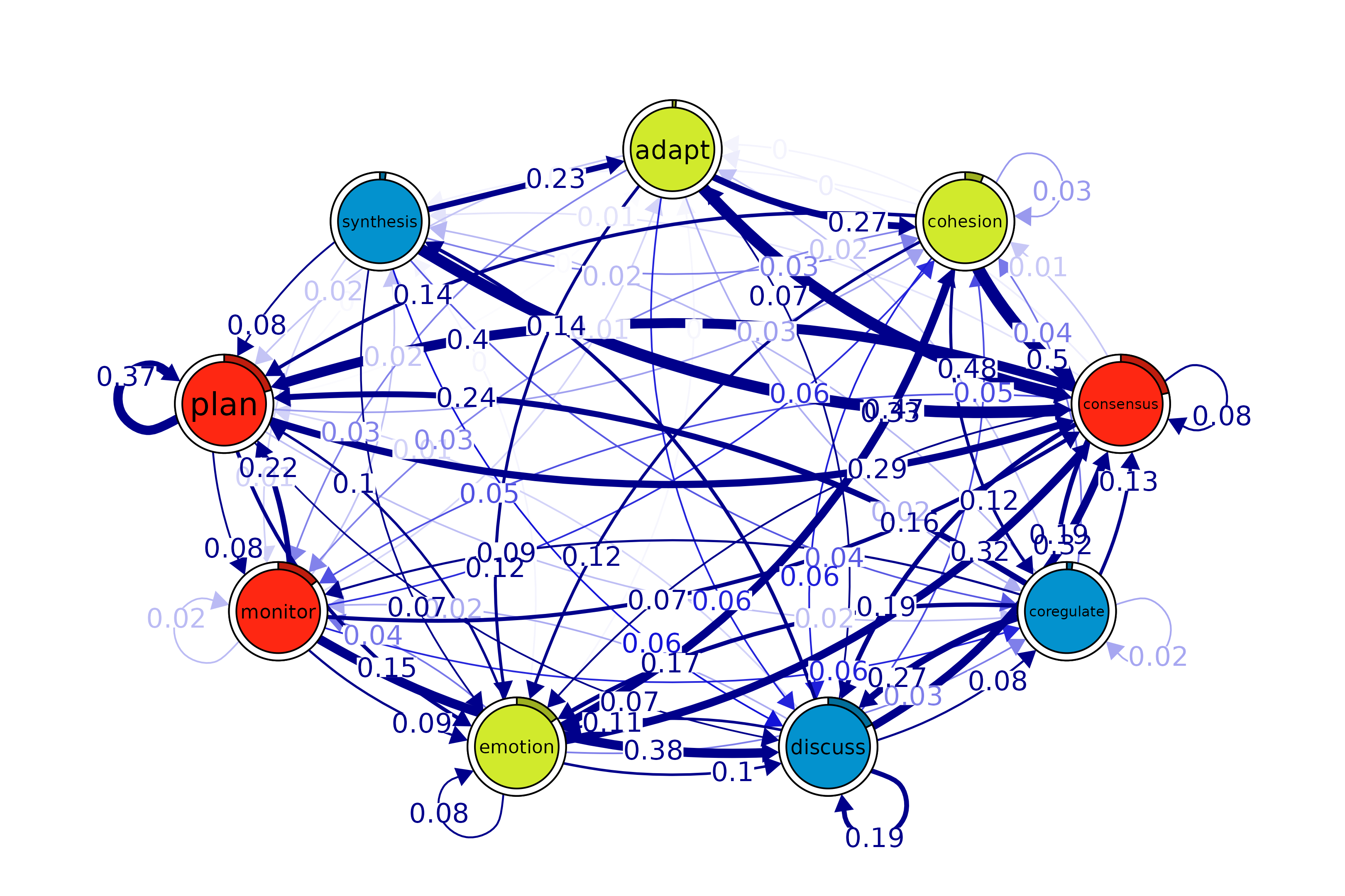
Network inference
Bootstrapping
# Perform bootstrapping on the TNA model with a fixed seed for reproducibility
set.seed(265)
boot <- bootstrap(model, threshold = 0.05)

# Print a summary of the bootstrap results
print(summary(boot))
#>         from    to weight p_value   sig cr_lower cr_upper ci_lower ci_upper
#> 2   cohesion adapt 0.0029    0.51 FALSE   0.0022   0.0037  0.00059   0.0054
#> 3  consensus adapt 0.0047    0.16 FALSE   0.0036   0.0059  0.00313   0.0065
#> 4 coregulate adapt 0.0162    0.15 FALSE   0.0122   0.0203  0.01078   0.0222
#>  [ reached 'max' / getOption("max.print") -- omitted 75 rows ]

# Show the non-significant edges (p-value >= 0.05 in this case)
# These are edges that are less likely to be stable across bootstrap samples
print(boot, type = "nonsig")
#> Non-significant Edges
#>
#>         from    to weight p_value cr_lower cr_upper ci_lower ci_upper
#> 2   cohesion adapt 0.0029    0.51   0.0022   0.0037  0.00059   0.0054
#> 3  consensus adapt 0.0047    0.16   0.0036   0.0059  0.00313   0.0065
#> 4 coregulate adapt 0.0162    0.15   0.0122   0.0203  0.01078   0.0222
#>  [ reached 'max' / getOption("max.print") -- omitted 24 rows ]
Permutation
# Create TNA for the high-achievers subset (rows 1 to 1000)
Hi <- tna(group_regulation[1:1000, ])

# Create TNA for the low-achievers subset (rows 1001 to 2000)
Lo <- tna(group_regulation[1001:2000, ])

# Plot a comparison of the "Hi" and "Lo" models
# The 'minimum' parameter is set to 0.001, so edges with weights >= 0.001 are shown
plot_compare(Hi, Lo, minimum = 0.01)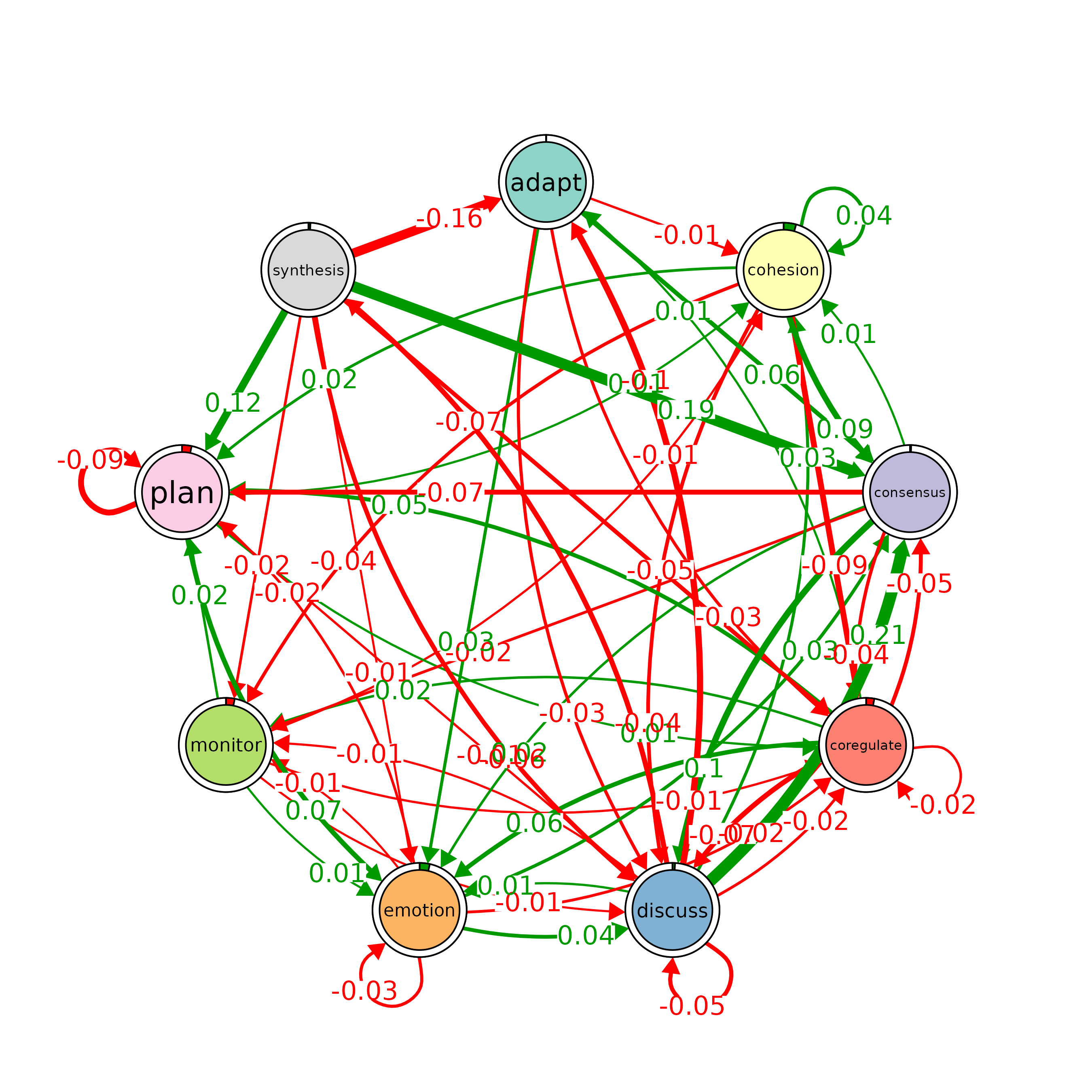
# Run a permutation test to determine statistical significance of differences
# between "Hi" and "Lo"
# The 'iter' argument is set to 1000, meaning 1000 permutations are performed
Permutation <- permutation_test(Hi, Lo, iter = 1000, measures = "Betweenness")

# Plot the significant differences identified in the permutation test
plot(Permutation, minimum = 0.01)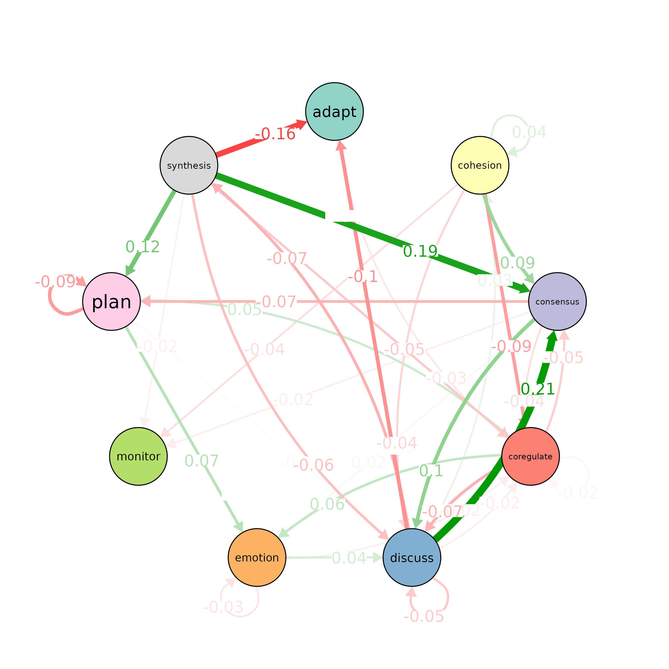
print(Permutation$edges$stats)
#> edge_name diff_true effect_size p_value
#> 1 adapt -> adapt 0.00000 NaN 1.000
#> 2 cohesion -> adapt 0.00533 1.991 0.061
#> 3 consensus -> adapt -0.00132 -0.763 0.412
#> 4 coregulate -> adapt 0.01122 2.002 0.048
#> 5 discuss -> adapt -0.09616 -11.482 0.001
#> 6 emotion -> adapt 0.00167 0.907 0.460
#> 7 monitor -> adapt -0.00019 -0.034 0.943
#> [ reached 'max' / getOption("max.print") -- omitted 74 rows ]
print(Permutation$centralities$stats)
#> state centrality diff_true effect_size p_value
#> 1 adapt Betweenness -3 -6.69 0.001
#> 2 cohesion Betweenness 0 0.00 1.000
#> 3 consensus Betweenness 5 7.01 0.001
#> 4 coregulate Betweenness -3 -0.97 0.265
#> 5 discuss Betweenness 2 1.83 0.233
#> 6 emotion Betweenness 2 16.33 0.001
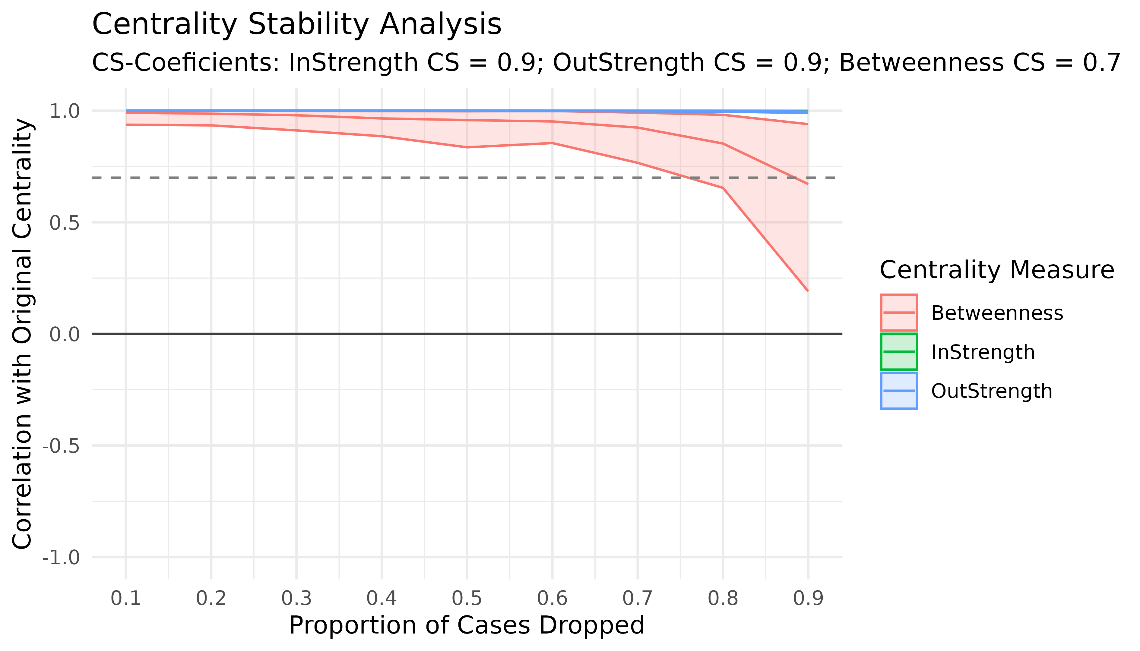
#> [ reached 'max' / getOption("max.print") -- omitted 3 rows ]Interpreting the Results of the Case-Dropping Bootstrap for Centrality Indices
# Results of the Case-Dropping Bootstrap for Centrality Indices
Centrality_stability <- estimate_centrality_stability(model, iter = 100)
plot(Centrality_stability)