Introduction to cograph

library(cograph)

Why cograph

R has several network packages — igraph for graph algorithms, qgraph for psychometric networks, tidygraph for dplyr-style manipulation. Each does one thing well but forces you into its own data format and API. Going from a raw matrix to a filtered, annotated, publication-ready figure typically means loading three packages, converting between formats, and writing boilerplate code to stitch the results together.

cograph was designed to eliminate that friction. Every function — plotting, centrality, community detection, filtering — accepts any major network format directly: matrices, edge lists, igraph, statnet, qgraph, and tna objects. No manual conversion. Centrality returns a tidy data frame, not a list of separate calls. Community detection is one function with 11 algorithms behind it. Statistical annotations (confidence intervals, p-values, significance stars) render directly on the figure. And when you need igraph or statnet for something cograph does not do, to_igraph() and to_network() convert back without data loss.

Beyond standard network analysis, cograph visualizes higher-order sequential pathways as simplicial blob diagrams, renders bootstrap stability results with forest plots (linear, circular, and grouped layouts), and performs motif analysis that identifies specific named node triples — not just abstract type counts.

The result is a single package that covers the full workflow from data import to publication-ready output, while remaining interoperable with the rest of the R network ecosystem.

set.seed(42)
n <- 10
states <- c("Explore", "Plan", "Monitor", "Adapt", "Reflect",
            "Discuss", "Synthesize", "Evaluate", "Create", "Share")
mat <- matrix(0, n, n, dimnames = list(states, states))
# Sparse: ~30% of edges populated
edges <- sample(which(row(mat) != col(mat)), 30)
mat[edges] <- round(runif(30, 0.05, 0.5), 2)

Plotting

splot() is the main plotting function. One call, publication-ready output.

splot(mat, tna_styling = TRUE, minimum = 0.1,
  title = "Learning Regulation Network")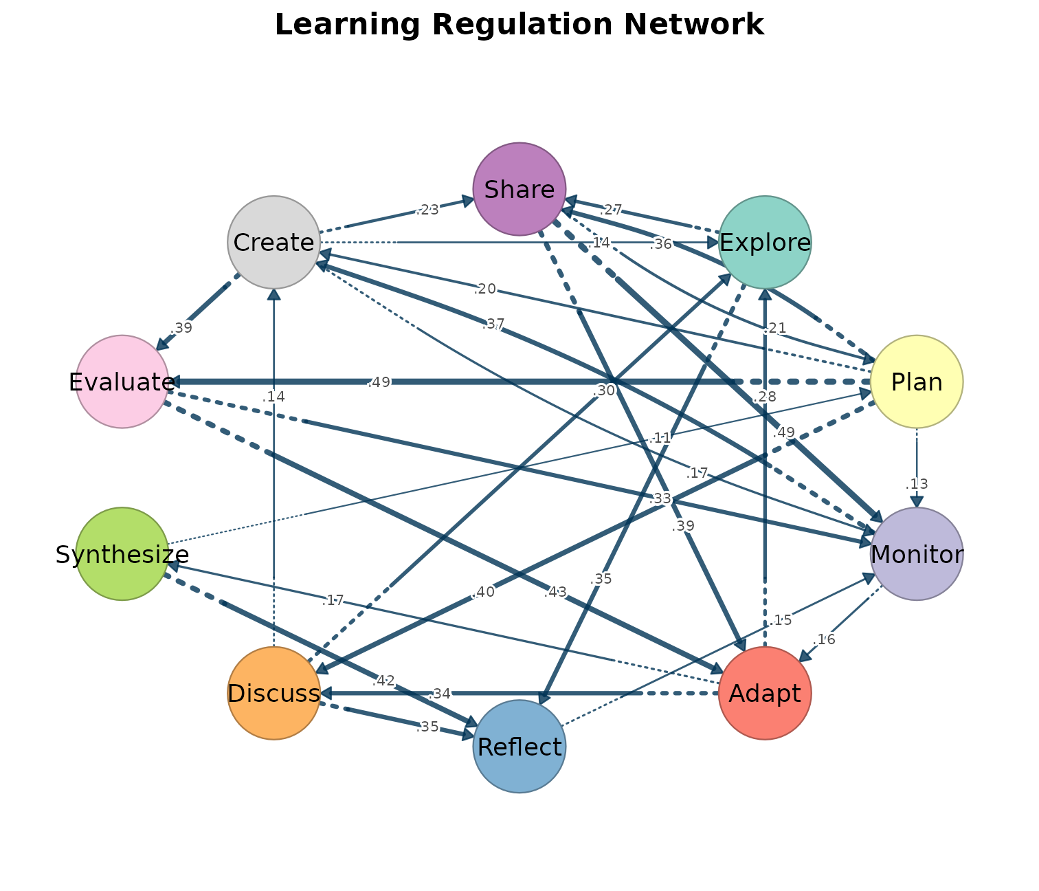

Key parameters: layout, minimum, node_fill, node_size, edge_labels, curvature, scale_nodes_by, theme, tna_styling.

splot(mat, layout = "spring")
splot(mat, minimum = 0.1, edge_labels = TRUE)
splot(mat, scale_nodes_by = "betweenness")
splot(mat, theme = "dark")
splot(mat, tna_styling = TRUE)

Layouts: "oval", "spring", "circle", "grid", "mds", "star", "bipartite", "groups", or a custom coordinate matrix.

Themes: "default", "dark", "minimal", "gray", "nature", "colorblind", "viridis".

Node shapes: "circle", "square", "triangle", "diamond", "pentagon", "hexagon", "star", "heart", "ellipse", "cross", "rectangle", "pie", "donut", or custom SVG via register_svg_shape().

Specialized plots

Function	Purpose
`splot()`	Network graph (base R)
`soplot()`	Grid/ggplot2 network
`plot_tna()` / `tplot()`	TNA-style wrappers with qgraph-compatible parameters
`plot_chord()`	Chord diagram (directed/undirected ribbons)
`plot_heatmap()`	Adjacency heatmap with clustering
`plot_ml_heatmap()`	Multi-layer comparison heatmap
`plot_transitions()` / `plot_alluvial()`	Alluvial / Sankey flow diagrams
`plot_trajectories()`	Individual trajectory tracking
`plot_compare()`	Difference network between two matrices
`plot_comparison_heatmap()`	Side-by-side heatmap comparison
`plot_mixed_network()`	Directed + undirected edges combined
`plot_bootstrap_forest()`	Bootstrap CI forest plots (linear, circular, grouped)
`plot_edge_diff_forest()`	Edge difference plots (linear, circular, chord, tile)
`plot_simplicial()`	Higher-order pathway blob overlays
`overlay_communities()`	Community blob overlays on network
`plot_mcml()`	Two-layer hierarchical cluster visualization
`plot_mtna()`	Flat multi-cluster layout
`plot_mlna()`	Stacked multilayer 3D perspective
`plot_htna()`	Multi-group heterogeneous TNA layout
`plot_robustness()`	Robustness degradation curves
`plot_permutation()` / `plot_group_permutation()`	Permutation test results

plot_simplicial(mat,
  c("Explore Plan -> Monitor",
    "Monitor Adapt -> Reflect",
    "Discuss Synthesize -> Evaluate",
    "Create Share -> Explore"),
  dismantled = TRUE, ncol = 2,
  title = "Higher-Order Pathways")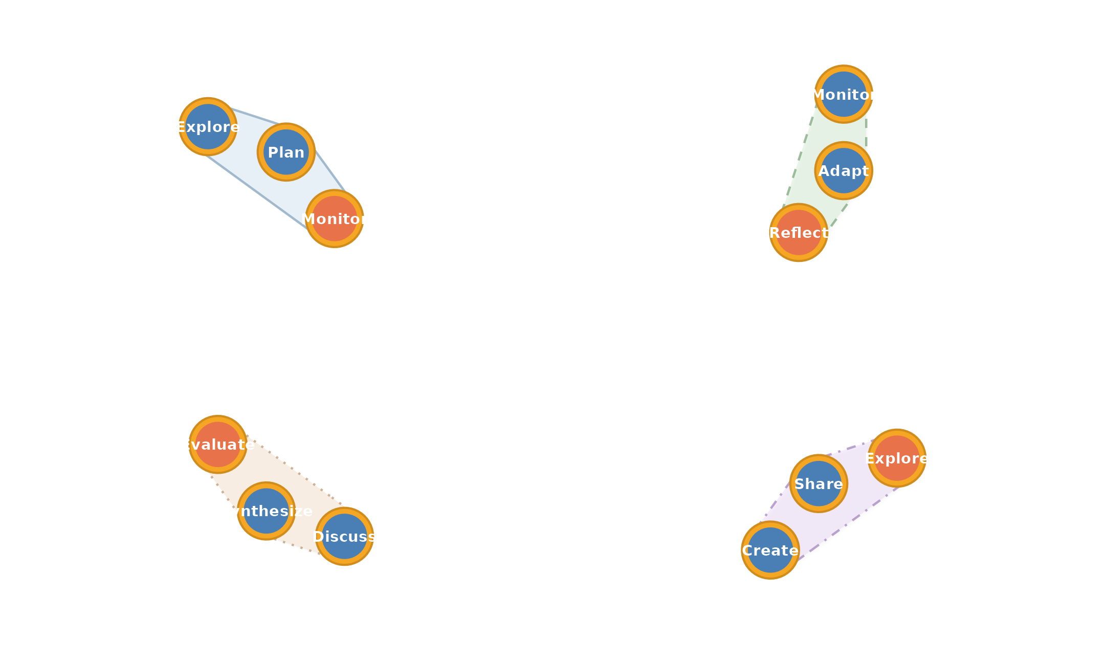

Input formats

Every function accepts six formats directly.

Format	Example
Matrix	`splot(mat)`
Edge list	`splot(data.frame(from = "A", to = "B", weight = 1))`
igraph	`splot(igraph::make_ring(5))`
statnet	`splot(network::network(mat))`
qgraph	`from_qgraph(q)`
tna	`splot(tna::tna(data))`

Conversion utilities:

Function	Output
`as_cograph(x)`	cograph_network object
`to_igraph(x)`	igraph object
`to_matrix(x)`	Adjacency matrix
`to_data_frame(x)` / `to_df(x)`	Edge list data frame
`to_network(x)`	statnet network object
`from_qgraph(q)`	Extract qgraph styles into cograph

Filtering and selection

Filter edges and nodes with expressions. Centrality measures are lazy-computed inside filter_nodes().

strong <- filter_edges(mat, weight > 0.3)
get_edges(strong)
#>    from to weight
#> 1     8  3   0.33
#> 2    10  3   0.49
#> 3     8  4   0.43
#> 4    10  4   0.39
#> 5     1  5   0.35
#> 6     6  5   0.35
#> 7     7  5   0.42
#> 8     2  6   0.40
#> 9     4  6   0.34
#> 10    2  8   0.49
#> 11    9  8   0.39
#> 12    3  9   0.37
#> 13    2 10   0.36

top3 <- select_nodes(mat, top = 3, by = "betweenness")
get_labels(top3)
#> [1] "Plan"    "Monitor" "Adapt"

Function	Purpose
`filter_edges(x, ...)`	Filter by weight, from, to
`filter_nodes(x, ...)`	Filter by degree, centrality, label
`select_nodes(x, ...)`	Top-N by centrality, by name, neighbors
`select_edges(x, ...)`	Top-N, involving, between, bridges, mutual
`select_neighbors(x, of)`	Ego-network extraction (multi-hop)
`select_component(x)`	Largest or named component
`select_top(x, n, by)`	Top-N nodes by any centrality
`select_bridges(x)`	Bridge edges only
`select_top_edges(x, n)`	Top-N edges by weight
`select_edges_involving(x, nodes)`	Edges touching specific nodes
`select_edges_between(x, s1, s2)`	Edges between two node sets
`subset_nodes(x, ...)` / `subset_edges(x, ...)`	Base R-style subsetting
`simplify(x)`	Remove multi-edges and self-loops

Getters and setters:

Function	Purpose
`get_nodes(x)` / `set_nodes(x, df)`	Node data frame
`get_edges(x)` / `set_edges(x, df)`	Edge data frame
`get_labels(x)`	Node label vector
`n_nodes(x)` / `n_edges(x)`	Counts
`is_directed(x)`	Directedness
`set_groups(x)` / `get_groups(x)`	Group assignments
`set_layout(x, layout)`	Layout coordinates
`summarize_network(x)`	Network summary

Centrality

centrality() computes up to 25 measures and returns a data frame.

centrality(mat, measures = c("degree", "betweenness", "pagerank"))
#>          node degree_all betweenness   pagerank
#> 1     Explore          6         5.0 0.11846147
#> 2        Plan          7        15.5 0.03640953
#> 3     Monitor          8        18.0 0.18376724
#> 4       Adapt          6        15.0 0.12356096
#> 5     Reflect          6        10.0 0.12513119
#> 6     Discuss          5         0.5 0.06803638
#> 7  Synthesize          4         6.5 0.03760071
#> 8    Evaluate          5         3.0 0.07386400
#> 9      Create          7        13.0 0.13821279
#> 10      Share          6         9.0 0.09495573

Individual functions return named vectors:

centrality_degree(mat)
#>    Explore       Plan    Monitor      Adapt    Reflect    Discuss Synthesize 
#>          6          7          8          6          6          5          4 
#>   Evaluate     Create      Share 
#>          5          7          6
centrality_pagerank(mat)
#>    Explore       Plan    Monitor      Adapt    Reflect    Discuss Synthesize 
#> 0.11846147 0.03640953 0.18376724 0.12356096 0.12513119 0.06803638 0.03760071 
#>   Evaluate     Create      Share 
#> 0.07386400 0.13821279 0.09495573

All 25 measures:

Category	Functions
Degree	`centrality_degree()`, `centrality_strength()`, `centrality_indegree()`, `centrality_outdegree()`, `centrality_instrength()`, `centrality_outstrength()`
Path	`centrality_betweenness()`, `centrality_closeness()`, `centrality_harmonic()`, `centrality_eccentricity()` (each with in/out variants)
Spectral	`centrality_eigenvector()`, `centrality_pagerank()`, `centrality_authority()`, `centrality_hub()`, `centrality_alpha()`, `centrality_power()`, `centrality_subgraph()`
Structural	`centrality_coreness()`, `centrality_constraint()`, `centrality_transitivity()`, `centrality_laplacian()`
Flow	`centrality_current_flow_closeness()`, `centrality_current_flow_betweenness()`, `centrality_load()`
Spreading	`centrality_diffusion()`, `centrality_leverage()`, `centrality_kreach()`, `centrality_voterank()`, `centrality_percolation()`

Edge centrality: edge_centrality(), edge_betweenness().

Network properties

network_summary() computes up to 37 network-level metrics.

network_summary(mat)
#>   node_count edge_count density component_count diameter mean_distance min_cut
#> 1         10         30   0.333               1     0.97         0.435       1
#>   centralization_degree centralization_in_degree centralization_out_degree
#> 1                 0.123                    0.333                     0.222
#>   centralization_betweenness centralization_closeness centralization_eigen
#> 1                      0.149                    0.238                0.479
#>   transitivity reciprocity assortativity_degree hub_score authority_score
#> 1        0.423       0.111               -0.116        NA              NA

Function	Purpose
`network_summary()`	37 metrics (density, diameter, clustering, etc.)
`network_small_world()`	Small-world coefficient
`network_rich_club()`	Rich-club coefficient
`network_global_efficiency()`	Global efficiency
`network_local_efficiency()`	Local efficiency
`degree_distribution()`	Degree histogram
`network_girth()`	Shortest cycle
`network_radius()`	Minimum eccentricity
`network_bridges()`	Bridge edges
`network_cut_vertices()`	Articulation points
`network_vertex_connectivity()`	Minimum vertices to disconnect
`network_clique_size()`	Largest complete subgraph

Community detection

11 algorithms with a consistent interface.

comms <- communities(mat, method = "walktrap")
comms
#> Community structure (walktrap)
#>   Number of communities: 2 
#>   Modularity: 0.1976 
#>   Community sizes: 5, 5 
#>   Nodes: 10
community_sizes(comms)
#> [1] 5 5

Function	Algorithm	Alias
`community_louvain()`	Louvain modularity	`com_lv()`
`community_leiden()`	Leiden (improved Louvain)	`com_ld()`
`community_fast_greedy()`	Fast greedy	`com_fg()`
`community_walktrap()`	Random walk	`com_wt()`
`community_infomap()`	Information flow	`com_im()`
`community_label_propagation()`	Label propagation	`com_lp()`
`community_edge_betweenness()`	Edge betweenness	`com_eb()`
`community_leading_eigenvector()`	Leading eigenvector	`com_le()`
`community_spinglass()`	Spin glass	`com_sg()`
`community_optimal()`	Exact optimization	`com_op()`
`community_fluid()`	Fluid communities	`com_fl()`

Additional community functions:

Function	Purpose
`community_consensus()`	Run algorithm N times, keep stable assignments
`compare_communities()`	Compare partitions (NMI, VI, Rand, adjusted Rand)
`modularity()`	Modularity score
`community_sizes()`	Size of each community
`color_communities()`	Color vector from community membership
`cluster_quality()`	Quality metrics (silhouette, Dunn index)
`cluster_significance()`	Permutation-based significance testing
`detect_communities()`	Alternative interface (returns data frame)

Motifs

Motif analysis identifies recurring 3-node patterns using the MAN classification (16 directed triad types).

mot <- motifs(mat, significance = FALSE)
mot
#> Motif Census 
#> Level: aggregate | States: 10 | Pattern: triangle 
#> 
#> Type distribution:
#> 
#> 030C 030T 120C 120D 120U 
#>    1    1    1    1    1 
#> 
#> Top 5 results:
#>  type count
#>  030T    11
#>  120C     3
#>  030C     2
#>  120D     2
#>  120U     1

Function	Purpose
`motifs()`	MAN type census with significance testing
`subgraphs()`	Named node triples forming each pattern
`motif_census()`	Low-level triad census
`extract_motifs()`	Per-individual motif extraction
`extract_triads()`	Extract specific triad types
`triad_census()`	Raw 16-type triad count
`get_edge_list()`	Edge list from tna for motif input

Plot types: plot(mot, type = "types"), "significance", "triads", "patterns".

Robustness

Simulate network degradation under targeted and random removal.

robustness(mat, type = "vertex", measure = "betweenness", n_iter = 100)
plot_robustness(x = mat, measures = c("betweenness", "degree", "random"))

Function	Purpose
`robustness()`	Simulate removal attacks (vertex or edge)
`plot_robustness()`	Plot robustness curves for multiple strategies
`robustness_summary()`	AUC and summary statistics
`robustness_auc()`	Area under the robustness curve

Disparity filter

Backbone extraction using the disparity filter (Serrano et al. 2009).

disparity_filter(mat)
splot.tna_disparity(disparity_filter(mat))

Multi-cluster visualization

clusters <- list(
  Cognitive  = c("Explore", "Plan", "Monitor", "Adapt", "Reflect"),
  Social     = c("Discuss", "Synthesize", "Share"),
  Evaluative = c("Evaluate", "Create")
)
plot_mcml(mat, clusters, mode = "tna")
plot_mtna(mat, clusters)

Function	Architecture
`plot_mcml()`	Two-layer: detail nodes + summary pies
`plot_mtna()`	Flat cluster layout
`plot_mlna()`	Stacked 3D multilayer
`plot_htna()`	Multi-group heterogeneous TNA
`cluster_summary()` / `build_mcml()`	Pre-compute cluster aggregation
`as_tna()` / `as_mcml()`	Convert cluster summaries to tna objects
`cluster_network()`	Extract cluster-level network

Multilayer networks

Construct and analyze supra-adjacency matrices for multilayer/multiplex networks.

Function	Purpose
`mlna()` / `supra_adjacency()`	Build supra-adjacency matrix
`supra_layer()` / `supra_interlayer()`	Extract individual layers
`aggregate_layers()` / `aggregate_weights()`	Combine layers
`plot_mlna()`	3D perspective visualization
`plot_ml_heatmap()`	Multi-layer heatmap comparison

Higher-order networks

Detect sequential dependencies beyond first-order Markov models. Requires the Nestimate package.

Function	Purpose
`build_hon()`	Higher-Order Network construction
`build_hypa()`	Path anomaly detection (hypergeometric null)
`build_mogen()`	Multi-order model selection (AIC/BIC)
`path_counts()`	k-step path frequencies
`plot_simplicial()`	Visualize pathways as blob overlays
`build_simplicial()`	Simplicial complex from cliques
`persistent_homology()`	Topological persistence across thresholds
`q_analysis()`	Multi-level structural connectivity
`verify_simplicial()`	Cross-validate via Euler-Poincare theorem

Nestimate integration

Nestimate estimates networks from sequence data. Its objects dispatch through splot() automatically.

library(Nestimate)
net <- build_network(data, method = "relative")
splot(net)

boot <- bootstrap_network(net, iter = 1000)
splot(boot)
plot_bootstrap_forest(boot)
plot_bootstrap_forest(boot, layout = "circular")
plot_bootstrap_forest(boot, layout = "grouped")

grp <- build_network(data, method = "relative", group = "condition")
splot(grp)

perm <- permutation_test(grp$A, grp$B, iter = 1000)
splot(perm)

Estimation methods: "relative", "frequency", "attention", "glasso", "pcor", "co_occurrence".

Object	splot() produces
`netobject`	Network plot (TNA styling)
`net_bootstrap`	Stability-styled (solid = stable, dashed = unstable)
`netobject_group`	Multi-panel grid (one per group)
`net_permutation`	Colored difference network
`boot_glasso`	GLASSO bootstrap stability
`wtna_mixed`	Mixed window TNA

TNA integration

Direct support for all tna package objects:

Object	What splot() does
`tna`	Network with donut rings, TNA styling
`group_tna`	Multi-panel grid per group
`tna_bootstrap`	Stability-styled edges
`tna_permutation`	Colored difference network
`group_tna_permutation`	Multi-panel permutation results
`tna_disparity`	Backbone filter visualization

Palettes

Function	Colors
`palette_viridis(n)`	Viridis scale
`palette_pastel(n)`	Soft pastel
`palette_blues(n)`	Blue gradient
`palette_reds(n)`	Red gradient
`palette_diverging(n)`	Blue-white-red
`palette_colorblind(n)`	Colorblind-safe
`palette_rainbow(n)`	Rainbow

Pipe API

The sn_* functions provide a chainable builder for the grid/ggplot2 rendering path.

mat |>
  cograph() |>
  sn_layout("spring") |>
  sn_theme("minimal") |>
  sn_nodes(size = 8, fill = "steelblue") |>
  sn_edges(curvature = 0.2) |>
  sn_render(title = "My Network")

mat |> cograph() |> sn_save("network.pdf")
p <- mat |> cograph() |> sn_ggplot()

Function	Purpose
`cograph()` / `as_cograph()`	Create network object
`sn_nodes()`	Node aesthetics
`sn_edges()`	Edge aesthetics
`sn_layout()`	Layout algorithm
`sn_theme()`	Visual theme
`sn_palette()`	Color palette
`sn_render()`	Render to screen
`sn_save()` / `sn_save_ggplot()`	Save to file
`sn_ggplot()`	Convert to ggplot2 object
`register_theme()` / `register_layout()` / `register_shape()`	Register custom themes, layouts, shapes

References:

Saqr, M., López-Pernas, S., Conde, M. A., & Hernández-García, A. (2024). Social Network Analysis: A Primer, a Guide and a Tutorial in R. In Learning Analytics Methods and Tutorials. Springer. https://doi.org/10.1007/978-3-031-54464-4_15
Saqr, M., López-Pernas, S., Conde, M. A., & Hernández-García, A. (2024). Community Detection: A Practical Guide to Unraveling Learning Communities. In Learning Analytics Methods and Tutorials. Springer. https://doi.org/10.1007/978-3-031-54464-4_16
Saqr, M., López-Pernas, S., Törmänen, T., Kaliisa, R., Misiejuk, K., & Tikka, S. (2025). Transition Network Analysis: A Novel Framework for Modeling, Visualizing, and Identifying the Temporal Patterns of Learners and Learning Processes. In Proceedings of the 15th LAK Conference (pp. 351–361). ACM. https://doi.org/10.1145/3706468.3706513
Tikka, S., López-Pernas, S., & Saqr, M. (2025). tna: An R Package for Transition Network Analysis. Applied Psychological Measurement. https://doi.org/10.1177/01466216251348840