Plot Centrality Stability Results

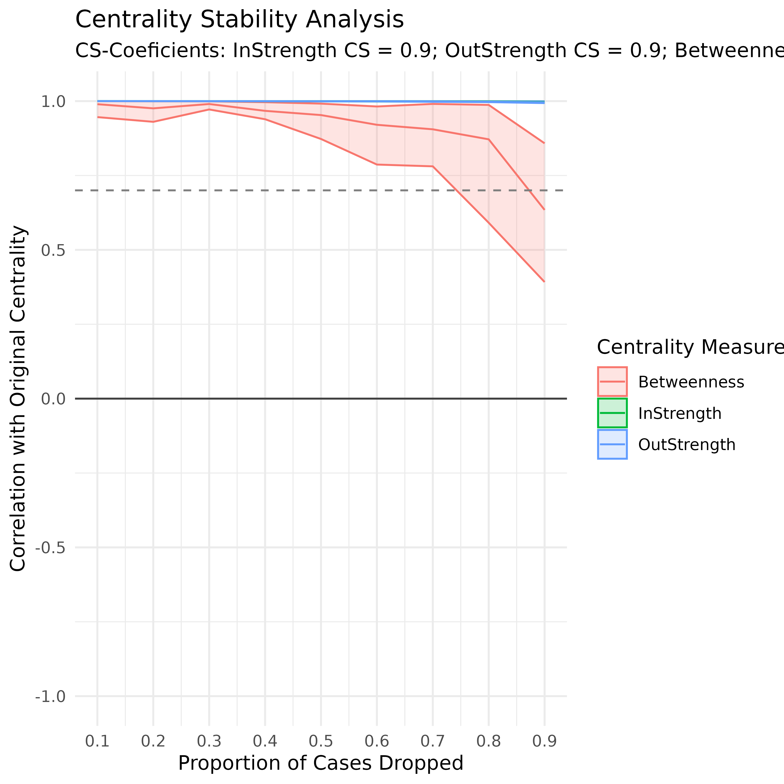
This function visualizes the centrality stability results produced by the estimate_centrality_stability function. It shows how different centrality measures' correlations change as varying proportions of cases are dropped, along with their confidence intervals (CIs).

Usage

# S3 method for class 'tna_stability'
plot(x, level = 0.05, ...)

Arguments

x

A tna_stability object produced by estimate_cs.

level

A numeric value representing the significance level for the confidence intervals. Defaults to 0.05.

...

Ignored.

Value

A ggplot object displaying the stability analysis plot.

Details

The function aggregates the results for each centrality measure across multiple proportions of dropped cases (e.g., 0.1, 0.2, ..., 0.9) and calculates the mean and the desired quantiles for each proportion. The confidence intervals (CIs) are computed based on the quantiles and displayed in the plot.

If no valid data is available for a centrality measure (e.g., missing or NA values), the function skips that measure with a warning.

The plot includes:

• The mean correlation for each centrality measure as a function of the proportion of dropped cases.

• Shaded confidence intervals representing CIs for each centrality measure.

• A horizontal dashed line at the threshold value used for calculating the CS-coefficient.

• A subtitle listing the CS-coefficients for each centrality measure.

See also

Validation functions bootstrap(), deprune(), estimate_cs(), permutation_test(), plot.group_tna_stability(), plot.tna_permutation(), print.group_tna_bootstrap(), print.group_tna_stability(), print.summary.group_tna_bootstrap(), print.summary.tna_bootstrap(), print.tna_bootstrap(), print.tna_permutation(), print.tna_stability(), prune(), pruning_details(), reprune(), summary.group_tna_bootstrap(), summary.tna_bootstrap()

Examples

model <- tna(group_regulation)
cs <- estimate_cs(model, iter = 10)
plot(cs)